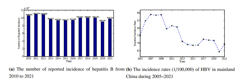
Figure 1.
The incidence of hepatitis B in mainland China, reported by China CDC [3].
Citation: Md. Hasan Ali, Robiul Islam Rubel. A comparative review of Mg/CNTs and Al/CNTs composite to explore the prospect of bimetallic Mg-Al/CNTs composites[J]. AIMS Materials Science, 2020, 7(3): 217-243. doi: 10.3934/matersci.2020.3.217
| [1] | Kangbo Bao, Qimin Zhang, Xining Li . A model of HBV infection with intervention strategies: dynamics analysis and numerical simulations. Mathematical Biosciences and Engineering, 2019, 16(4): 2562-2586. doi: 10.3934/mbe.2019129 |
| [2] | Tingting Xue, Long Zhang, Xiaolin Fan . Dynamic modeling and analysis of Hepatitis B epidemic with general incidence. Mathematical Biosciences and Engineering, 2023, 20(6): 10883-10908. doi: 10.3934/mbe.2023483 |
| [3] | Tailei Zhang, Hui Li, Na Xie, Wenhui Fu, Kai Wang, Xiongjie Ding . Mathematical analysis and simulation of a Hepatitis B model with time delay: A case study for Xinjiang, China. Mathematical Biosciences and Engineering, 2020, 17(2): 1757-1775. doi: 10.3934/mbe.2020092 |
| [4] | Maysaa Al Qurashi, Saima Rashid, Fahd Jarad . A computational study of a stochastic fractal-fractional hepatitis B virus infection incorporating delayed immune reactions via the exponential decay. Mathematical Biosciences and Engineering, 2022, 19(12): 12950-12980. doi: 10.3934/mbe.2022605 |
| [5] | Fathalla A. Rihan, Hebatallah J. Alsakaji . Analysis of a stochastic HBV infection model with delayed immune response. Mathematical Biosciences and Engineering, 2021, 18(5): 5194-5220. doi: 10.3934/mbe.2021264 |
| [6] | Dong-Me Li, Bing Chai, Qi Wang . A model of hepatitis B virus with random interference infection rate. Mathematical Biosciences and Engineering, 2021, 18(6): 8257-8297. doi: 10.3934/mbe.2021410 |
| [7] | Dwi Lestari, Noorma Yulia Megawati, Nanang Susyanto, Fajar Adi-Kusumo . Qualitative behaviour of a stochastic hepatitis C epidemic model in cellular level. Mathematical Biosciences and Engineering, 2022, 19(2): 1515-1535. doi: 10.3934/mbe.2022070 |
| [8] | Suxia Zhang, Hongbin Guo, Robert Smith? . Dynamical analysis for a hepatitis B transmission model with immigration and infection age. Mathematical Biosciences and Engineering, 2018, 15(6): 1291-1313. doi: 10.3934/mbe.2018060 |
| [9] | Sarah Kadelka, Stanca M Ciupe . Mathematical investigation of HBeAg seroclearance. Mathematical Biosciences and Engineering, 2019, 16(6): 7616-7658. doi: 10.3934/mbe.2019382 |
| [10] | Xiaojing Wang, Yu Liang, Jiahui Li, Maoxing Liu . Modeling COVID-19 transmission dynamics incorporating media coverage and vaccination. Mathematical Biosciences and Engineering, 2023, 20(6): 10392-10403. doi: 10.3934/mbe.2023456 |
Hepatitis B, a viral liver infection caused by the hepatitis B virus (HBV), is a major threat to public health and security around the whole world. HBV can cause both acute and chronic hepatitis. Acute hepatitis B refers to the virus infection less than half a year and part of the patients can recover and get lifetime immunity. The disease course of chronic hepatitis B can be quite long, and it can lead to severe liver disease such as cirrhosis and liver cancer [1]. Globally 257 million people were living with chronic hepatitis B infection, which resulted in estimated 887,000 deaths in 2015. According to the latest fact sheets released by the World Health Organization (WHO), 296 million people were living with chronic hepatitis B infection in 2019, and there are 1.5 million new infections each year [2]. Worldwide, hepatitis B resulted in an estimated 820,000 deaths in 2019, mostly from cirrhosis and hepatocellular carcinoma (primary liver cancer) [2]. Hence, hepatitis B epidemic is still a major global health problem.
In China, hepatitis B is one of the top three infectious diseases reported by the Chinese Center for Disease Control and Prevention (CDC) [3]. Based on the sero-epidemiological investigation of hepatitis B in 1992, about 9.75% of the general population in China was chronic HBV carriers. That is, around 130 million people of mainland China were carriers of HBV in the 1990s [1]. Then an effective and national vaccination program has been conducted by the government, especially the hepatitis B planned immunization for newborn babies and children. The sero-epidemiological survey in 2006 showed about 7.18% of the population was hepatitis B carriers, and the number of hepatitis B carriers was reduced by 30 million [3]. Lately in 2014, an epidemiology survey of people younger than 29 reported that the HBV infection rates were 0.32% among the group of children aged one to four, 0.94% in the group aged 5 to 14, and 4.18% in the group aged 15 to 29, respectively. The government of mainland China has achieved remarkable results in the prevention and treatment of hepatitis B. Nevertheless, the epidemic situation remains to be severe and complicated. At present there are 80 million HBV carriers in mainland China, among whom 28 million carriers need immediate medical treatment. During the past decade, the number of reported incidence of hepatitis B is around one million each year (Figure 1(a)). The incidence rates of hepatitis B in mainland China from 2005 to 2021 are presented in Figure 1(b), and the incidence rates varied from 89.00 per 100,000 in 2007 (the highest during 2005–2021) to 64.29 per 100,000 in 2020 (the lowest during 2005–2021).
The incidence of hepatitis B is different among regions, and it could be influenced by various factors such as vaccination and economy. Figure 2 displays the hepatitis B incidence rates in 31 provinces and municipalities of mainland China, and the data in 2007 and 2020 are chosen and displayed. The figure shows that the incidence decreased for most provinces (22 of 31), especially for Ningxia, Gansu, Henan, Xinjiang and Qinghai. This strongly reveals that the immunization program with hepatitis B vaccine is successful in most provinces, and the achievement is remarkable for western areas in China. However, it should be pointed out, in 2020, the incidence varied from 6.15 per 100,000 in Beijing to 150.99 per 100,000 in Qinghai. There is still a gap between the impoverished west and the prosperous east.

In the last three decades, the research on hepatitis B has attracted more and more attention from the perspective of epidemiology and biomathematics. For instance, in 1991, Anderson and May used a simple mathematical model to study the impacts of carriers on the transmission of HBV [4]. Zhao et al. [5] studied the dynamics of HBV transmission and proposed vaccination strategy to prevent the prevalence in the population. In 2010, Zou et al. [1] formulated a high dimensional deterministic model to analyze the transmission dynamics of HBV infection in China. Then in 2015 Zou et al. [6] investigated the sexual transmission dynamics of HBV in China. Zhang et al. [7] proposed a four dimensional HBV epidemic model involving an exponential birth rate and vertical transmission, and fitted the parameters to the public data in Xinjiang, China. Recently Din and Li [8] analyzed a stochastic hepatitis B epidemic model with vaccination effect and showed a case study for Pakistan. For more mathematical epidemic models on HBV infection, one can refer to [9,10,11,12] and the references therein.
Besides the classical compartmental models for hepatitis B epidemic, a vibrant field of research on the virus transmission dynamics has emerged and developed rapidly [12]. The modeling approaches usually incorporate the interaction among intracellular viral dynamics, multicellular infection process, and immune responses [13,14,15,16]. For instance, Wang et al. [13] formulated a multi-scale computational model of SARS-CoV-2 infection using a combination of differential equations and stochastic modeling, and revealed heterogeneity among COVID-19 patients. Rihan and Alsakaji [14] analyzed a stochastic delay HBV infection model with cell-to-cell transmission and cytotoxic T lymphocytes (CTLs) immune response. Recently Mohajerani et al. [17] proposed a multiscale modeling of HBV capsid assembly pathways, by constructing Markov state models and employing transition path theory.
When an infectious disease breaks out in one area, the center for disease control and prevention will release authoritative information through the mass media at the first moment, including the potential risk of the disease and prevention measures [18]. Media coverage helps to raise public health awareness, increase vaccine rates and reduce the spread of infections. Recently, a number of epidemic models have taken into account the influence of media coverage on the spread of infectious disease [19,20,21,22,23]. Their study suggests that media coverage is critical in disease eradication [19,20]. There are different forms of function to represent the effect of media coverage in epidemic models. Let S and I denote the number of the population that are susceptible and infectious respectively, and let β be the transmission rate. Cui et al. [19] used the exponential function βexp(−mI)SI to denote the incidence rate with media coverage, where m>0. In another work [20], the incidence rate incorporating media coverage takes the form: (β−β2f(I))SI, where β>β2 and the function f(I) satisfies f(0)=0, f′(I)≥0, limI→+∞f(I)=1. In the present paper, similar to the approach in the previous literatures [21,24,25], we adopt the most common form f(I)=Ib+I, where b is a half saturation constant.
Furthermore, the transmission of HBV is disturbed by various random factors in the environment, such as population mobility and unpredictable exposure to infections. An increasing number of researchers have formulated stochastic hepatitis B epidemic models considering environmental noise [8,10,11]. In fact, environment disturbances have an important effect on the evolution of infectious diseases [26,27,28,29,30], and Gaussian white noise is usually selected as an appropriate representation of environmental fluctuations [31]. For instance, Wang et al. [28] and Meng et al. [29] proved that a large disturbance of white noise can lead infectious diseases to extinction. A large number of works also indicate that stochastic disturbance can suppress disease outbreak [18,26].
In the present paper, motivated by the above discussion, we formulate and investigate a stochastic hepatitis B model with media coverage and saturated incidence rate. We obtain a sufficient condition for the extinction of the disease, and prove that the stochastic system has a unique stationary distribution under certain conditions. Moreover, as a case study, we utilize our model for fitting the available data of mainland China from 2005 to 2021. Based on our simulation result, the incidence rate of hepatitis B in China will remain around 50–60 per 100,000 in the long term.
The paper is organized as follows. In Section 2, we present the model formulation. In Section 3, the existence and uniqueness of positive solution is proved for the stochastic model. In Section 4, we obtain a sufficient condition for the extinction of the disease. In Section 5, the sufficient condition on the existence of stationary distribution is obtained, which indicates that all the compartments will be persistent. Moreover, we provide an estimation of lower bound of the expectation for the number of infected cases. In Section 6, numerical simulations are conducted to illustrate our theoretical results. As a case study, we fit our model to the available HBV data of mainland China from 2005 to 2021.
Recently, Khan et al. [10] proposed a stochastic model for the transmission of HBV. In their work, the population is divided into four compartments: susceptible humans S; acute HBV infections I1; chronical HBV infections I2; and recovered population R. They further assumed: (i) the contact of susceptible individuals with acutely and chronically infected hepatitis B individuals primarily causes acutely infected species; (ii) the transmission coefficient β is subject to random fluctuation, that is, βi→βi+ηi˙Bi(t) for i=1,2, where Bi(t) is standard Brownian motion with Bi(0)=0 and with the noise intensity η2i>0. Then the stochastic hepatitis B epidemic model in [10] was presented as follows
| {dS(t)=[Λ−2∑i=1βiS(t)Ii(t)−(μ0+υ)S(t)]dt−2∑i=1ηiS(t)Ii(t)dBi(t),dI1(t)=[2∑i=1βiS(t)Ii(t)−(μ0+γ+γ1)I1(t)]dt+2∑i=1ηiS(t)Ii(t)dBi(t),dI2(t)=[γI1(t)−(μ0+μ1+γ2)I2(t)]dt,dR(t)=[γ1I1(t)+γ2I2(t)+υS(t)−μ0R(t)]dt, | (2.1) |
where Λ is the recruitment rate of the population, μ0 is the natural mortality rate, μ1 is the disease mortality rate, and υ represents the vaccination rate of hepatitis B. Moreover, βi (i=1,2) represent the transmission rate of hepatitis B, γ is the moving rate of acutely infected humans to chronic stage, and γi (i=1,2) denote the recovery rates of acutely and chronically infected hepatitis B individuals, respectively.
In the above model, the authors chose bilinear incidence rate, that is, βSI. As a matter of fact, the transmission of infectious diseases is complicated, and nonlinear incidence rates have been wildly utilized in epidemic model [26,29]. In 1978, to describe the phenomenon that incidence is increasing and the population is saturated with the infective, Capasso and Serio [32] proposed a saturated incidence rate βSI1+αI. Then such saturated incidence has been extensively used in epidemic models. For instance, Khan and Zaman [33] and Liu et al. [11] have formulated hepatitis B epidemic models with saturated incidence rate. In addition, as discussed in the introduction part, we also incorporate the impact of media coverage by using the function f(I)=Ib+I. Consequently, based on the deterministic part of model (2.1), we obtain the hepatitis B model with media coverage and saturated incidence rate as follows
| {dS(t)dt=Λ−(β11−β12I1(t)b1+I1(t))S(t)I1(t)1+α1I1(t)−(β21−β22I2(t)b2+I2(t))S(t)I2(t)1+α2I2(t)−(μ0+υ)S(t),dI1(t)dt=(β11−β12I1(t)b1+I1(t))S(t)I1(t)1+α1I1(t)+(β21−β22I2(t)b2+I2(t))S(t)I2(t)1+α2I2(t)−(μ0+γ+γ1)I1(t),dI2(t)dt=γI1(t)−(μ0+μ1+γ2)I2(t),dR(t)dt=γ1I1(t)+γ2I2(t)+υS(t)−μ0R(t), | (2.2) |
where the forms SIi1+αiIi (i=1,2) represent the saturated incidence rates of acute and chronical infections, and the forms Iibi+Ii (i=1,2) denote the media coverage functions. Moreover, βi1 (i=1,2) represent the transmission rates for acute and chronical infections, and βi2 (i=1,2) denote the maximal reduced contact rates by mass media alert for acute and chronical infections, respectively. Recall that βi1>βi2 (i=1,2).
Furthermore, the disease transmission and biological populations are inevitably affected by environment noises. There are different approaches to add random perturbations to biological systems. The transmission rates βi (i=1,2) are assumed to be disturbed by Gaussian white noise in model (2.1). In this article, following the approach in [8,11,34,35], we assume that the environmental white noise is proportional to each state variable S(t),I1(t),I2(t) and R(t). Finally we extend model (2.2) to the following stochastic model
| {dS(t)=[Λ−(β11−β12I1b1+I1)SI11+α1I1−(β21−β22I2b2+I2)SI21+α2I2−(μ0+υ)S]dt+σ1SdB1(t),dI1(t)=[(β11−β12I1b1+I1)SI11+α1I1+(β21−β22I2b2+I2)SI21+α2I2−(μ0+γ+γ1)I1]dt+σ2I1dB2(t),dI2(t)=[γI1−(μ0+μ1+γ2)I2]dt+σ3I2dB3(t),dR(t)=[γ1I1+γ2I2+υS−μ0R]dt+σ4RdB4(t), | (2.3) |
where Bi(t) (i=1,2,3,4) are independent standard Brownian motions with Bi(0)=0, and σ2i>0 (i=1,2,3,4) denote the intensities of white noise.
Throughout the paper, let (Ω,F,{Ft}t≥0,P) be a complete probability space with a filtration {Ft}t≥0 satisfying the usual conditions (i.e., it is increasing and right continuous while F0 contains all P-null sets), then Bi(t) (i=1,2,3,4) are defined on this complete probability space. We also introduce the following notations: Rd+={(x1,x2,...,xd)∈Rd:xi>0,i=1,2,...,d}, a∧b=min{a,b}, a∨b=max{a,b}, ⟨f⟩=1t∫t0f(r)dr.
Since S,I1,I2 and R in system (2.3) denote the number of individuals, they should be nonnegative from the viewpoint of biology. We first introduce some basic definitions that will be used in the reminder of the article [36]. In general, let X(t) be a homogeneous Markov process in the d-dimension Euclidean space Rd described by the stochastic differential equation
| dX(t)=f(X)dt+k∑r=1σr(X)dBr(t), | (3.1) |
then the diffusion matrix is defined as
| A(x)=(aij(x)),aij(x)=k∑r=1σir(x)σjr(x). |
Furthermore, the differential operator L is defined by
| LV(x)=d∑i=1fi(x)∂V(x)∂xi+12d∑i,j=1aij(x)∂2V(x)∂xi∂xj, |
where V(x) is an arbitrary twice continuously differential real-value function.
In this section, we obtain the following theorem which guarantees the existence and uniqueness of positive solution for system (2.3).
Theorem 3.1. For any initial value (S(0),I1(0),I2(0),R(0))∈R4+, there is a unique positive solution (S(t),I1(t),I2(t),R(t)) for system (2.3) on t≥0 and the solution will remain in R4+ with probability one, namely, (S(t),I1(t),I2(t),R(t))∈R4+ for all t≥0 almost surely.
Proof. Since the coefficients of system (2.3) are locally Lipschitz continuous in R4+, then for any initial value (S(0),I1(0),I2(0),R(0))∈R4+, there exists a unique positive solution (S(t),I1(t),I2(t),R(t)) on t∈[0,τe), where τe is the explosion time [37]. Thus, it suffices to verify S(t), I1(t), I2(t) and R(t) do not explode to infinity in a finite time, that is, τe=∞ a.s. Let k0>0 be sufficiently large such that S(0), I1(0), I2(0) and R(0) all lie within the interval [1k0,k0]. For each integer k≥k0, define the stopping time
| τk=inf{t∈[0,τe):min{S(t),I1(t),I2(t),R(t)}≤1kormax{S(t),I1(t),I2(t),R(t)}≥k}, |
and throughout this paper we set inf∅=∞ (as usual ∅ is the empty set). Clearly, τk is increasing as k→∞. Let τ∞=limk→∞τk, then τ∞≤τe a.s. Thus, τ∞=∞ a.s. implies τe=∞ a.s. Now we state that τ∞=∞. If this assertion is false, then there is a pair of constants T>0 and ϵ∈(0,1) such that
| P{τ∞≤T}>ϵ. |
Thus there exists an integer k1≥k0 such that
| P{τk≤T}≥ϵfor allk≥k1. | (3.2) |
Define a C2-function V:R4+→R+ by
| V(S,I1,I2,R)=(S−a−alnSa)+(I1−b−blnI1b)+(I2−1−lnI2)+(R−1−lnR), |
where a and b are positive constants to be determined later. The nonnegativity of this function can be obtained from
| v−1−lnv≥0for anyv>0. |
Apply Itô's formula [37] to V, and we obtain
| dV(S,I1,I2,R)=LV(S,I1,I2,R)dt+σ1(S−a)dB1(t)+σ2(I1−b)dB2(t)+σ3(I2−1)dB3(t)+σ4(R−1)dB4(t), | (3.3) |
where
| LV=(1−aS)[Λ−(β11−β12I1b1+I1)SI11+α1I1−(β21−β22I2b2+I2)SI21+α2I2−(μ0+υ)S]+aσ212+(1−bI1)[(β11−β12I1b1+I1)SI11+α1I1+(β21−β22I2b2+I2)SI21+α2I2−(μ0+γ+γ1)I1]+bσ222+(1−1I2)[γI1−(μ0+μ1+γ2)I2]+σ232+(1−1R)[γ1I1+γ2I2+υS−μ0R]+σ242=Λ−μ0S−aΛS+a(β11−β12I1b1+I1)I11+α1I1+a(β21−β22I2b2+I2)I21+α2I2+a(μ0+υ+σ212)−μ0I1−b(β11−β12I1b1+I1)S1+α1I1−b(β21−β22I2b2+I2)SI2I1(1+α2I2)+b(μ0+γ+γ1+σ222)−(μ0+μ1)I2−γI1I2+μ0+μ1+γ2+σ232−μ0R−γ1I1R−γ2I2R−υSR+μ0+σ242≤Λ−μ0S−μ0I1−(μ0+μ1)I2+aβ11I11+α1I1+aβ21I21+α2I2+a(μ0+υ+σ212)+bβ12I1S(b1+I1)(1+α1I1)+b(μ0+γ+γ1+σ222)+2μ0+μ1+γ2+σ232+σ242≤Λ−μ0S−μ0I1−(μ0+μ1)I2+aβ11I1+aβ21I2+a(μ0+υ+σ212)+bβ12Sb1α1+b(μ0+γ+γ1+σ222)+2μ0+μ1+γ2+σ232+σ242=Λ+(bβ12b1α1−μ0)S+(aβ11−μ0)I1+(aβ21−μ0−μ1)I2+a(μ0+υ+σ212)+b(μ0+γ+γ1+σ222)+2μ0+μ1+γ2+σ232+σ242. |
Choose a=min{μ0β11,μ0+μ1β21} and b=μ0b1α1β12, then
| aβ11−μ0≤0,aβ21−μ0−μ1≤0andbβ12b1α1−μ0=0, |
and
| LV(S,I1,I2,R)≤Λ+a(μ0+υ+σ212)+b(μ0+γ+γ1+σ222)+2μ0+μ1+γ2+σ232+σ242:=K, |
where K is a positive number. Thus, according to Eq (3.3), one can get
| dV(S,I1,I2,R)≤Kdt+σ1(S−a)dB1(t)+σ2(I1−b)dB2(t)+σ3(I2−1)dB3(t)+σ4(R−1)dB4(t). |
Let k≥k1 and integrate the above inequality from 0 to τk∧T, then we have
| ∫τk∧T0dV(S,I1,I2,R)≤∫τk∧T0Kdt+∫τk∧T0σ1(S−a)dB1(t)+∫τk∧T0σ2(I1−b)dB2(t)+∫τk∧T0σ3(I2−1)dB3(t)+∫τk∧T0σ4(R−1)dB4(t). | (3.4) |
Taking the expectation of both sides of Eq (3.4) yields
| E(V(S(τk∧T),I1(τk∧T),I2(τk∧T),R(τk∧T)))≤V(S(0),I1(0),I2(0),R(0))+KT. | (3.5) |
Set Ωk={ω∈Ω:τk=τk(ω)≤T} for k≥k1, then we have P(Ωk)≥ϵ by (3.2). Note that for every ω∈Ωk, at least one of S(τk,ω),I1(τk,ω),I2(τk,ω) and R(τk,ω) equals to either k or 1k, So V(S(τk,ω),I1(τk,ω),I2(τk,ω),R(τk,ω)) is no less than either
| k−1−lnkor1k−1−ln1korn−a−alnkaor1k−a+aln(ka)ork−b−blnkbor1k−b+bln(kb). |
Thus, one can obtain
| V(S(τk),I1(τk),I2(τk),R(τk))≥(k−1−lnk)∧(1k−1−ln1k)∧(k−a−alnka)∧(1k−a+aln(ka))∧(k−b−blnkb)∧(1k−b+bln(kb)). |
It then follows from Eq (3.5) that
| ∞>V(S(0),I1(0),I2(0),R(0))+KT≥E(IΩn(ω)V(S(τk),I1(τk),I2(τk),R(τk))=P(Ωk)V(S(τk),I1(τk),I2(τk),R(τk))≥ϵV(S(τk),I1(τk),I2(τk),R(τk))≥ϵ[(k−1−lnk)∧(1k−1−ln1k)∧(k−a−alnka)∧(1k−a+aln(ka))∧(k−b−blnkb)∧(1k−b+bln(kb))], |
where IΩk(ω) is the indicator function of Ωk. Taking k→∞ will induce ∞>V(S(0),I1(0),I2(0),R(0))+KT≥+∞, and it is a contradiction. Hence, we must have τ∞=∞ a.s.
The conclusion is confirmed.
In this section, we mainly discuss the extinction of hepatitis B under some conditions. To begin with, we present the following theorem.
Theorem 4.1. If min{μ0,μ1}>(σ21∨σ22∨σ23∨σ24)2, then the solution (S(t),I2(t),Sh(t),Ih(t)) of system (2.3) has the following properties
| limt→∞S(t)t=0,limt→∞I1(t)t=0,limt→∞I2(t)t=0,limt→∞R(t)t=0a.s. |
and
| limt→∞∫t0S(s)dB1(s)t=0,limt→∞∫t0I1(s)dB2(s)t=0,limt→∞∫t0I2(s)dB3(s)t=0,limt→∞∫t0R(s)dB4(s)t=0a.s. |
The proof is similar to those in [38] and hence is omitted here.
It is easy to compute that the deterministic system (2.2) admits a disease-free equilibrium point E0(Λμ0+υ,0,0,Λυμ0(μ0+υ)). For the stochastic system (2.3), we obtain a sufficient condition on the extinction of disease in the following theorem.
Theorem 4.2. Let (S(t),I1(t),I2(t),R(t)) be a solution of system (2.3) with initial value (S(0), I1(0), I2(0), R(0))∈R4+. If Rs0:=4Λ(2β11−β12+2β21−β22)μ0(σ22∧σ23)<1 and min{μ0,μ1}>(σ21∨σ22∨σ23∨σ24)2 hold, then the disease will tend to extinction with probability one, and the solution of system (2.3) satisfies
| limt→∞I1(t)=0,limt→∞I2(t)=0,lim supt→∞⟨S(t)+R(t)⟩=Λμ0. |
Proof. Denote
| Q(t)=I1(t)+I2(t), |
and applying Itô's formula to lnQ yields
| dlnQ={1I1+I2[(β11−β12I1b1+I1)SI11+α1I1+(β21−β22I2b2+I2)SI21+α2I2−(μ0+γ1)I1−(μ0+μ1+γ2)I2]−12(I1+I2)2(σ22I21+σ23I22)}dt+σ2I1I1+I2dB2(t)+σ3I2I1+I2dB3(t)≤{(2β11−β12)S+(2β21−β22)S−σ22∧σ234(I21+I22)(I21+I22)}dt+σ2I1I1+I2dB2(t)+σ3I2I1+I2dB3(t)={(2β11−β12)S+(2β21−β22)S−σ22∧σ234}dt+σ2I1I1+I2dB2(t)+σ3I2I1+I2dB3(t). | (4.1) |
Integrate inequality (4.1) from 0 to t and divide by t on both sides, then we get
| lnQ(t)−lnQ(0)t≤(2β11−β12+2β21−β22)⟨S⟩−σ22∧σ234+σ2t∫t0I1I1+I2dB2(s)+σ3t∫t0I2I1+I2dB3(s). | (4.2) |
According to system (2.3), we have
| d(S+I1+I2+R)=[Λ−μ0(S+I1+I2+R)−μ1I2]dt+σ1SdB1(t)+σ2I1dB2(t)+σ3I2dB3(t)+σ4RdB4(t)≤[Λ−μ0(S+I1+I2+R)]dt+σ1SdB1(t)+σ2I1dB2(t)+σ3I2dB3(t)+σ4RdB4(t). | (4.3) |
Integrate the above inequality form 0 to t and divide by t on both sides, then
| S(t)+I1(t)+I2(t)+R(t)t−S(0)+I1(0)+I2(0)+R(0)t≤Λ−μ0t∫t0(S+I1+I2+R)ds+σ1∫t0S(s)dB1(s)t+σ2∫t0I1(s)dB2(s)t+σ3∫t0I2(s)dB3(s)t+σ4∫t0R(s)dB4(s)t. | (4.4) |
Furthermore, it follows from Theorem 4.1 that
| lim supt→∞⟨S+I1+I2+R⟩≤Λμ0a.s. | (4.5) |
Therefore,
| lim supt→∞⟨S⟩≤Λμ0a.s. | (4.6) |
Take the superior limit on both sides of inequality (4.2), then we have
| lim supt→∞lnQ(t)t≤(2β11−β12+2β21−β22)Λμ0−σ22∧σ234=σ22∧σ234(Rs0−1)<0a.s. |
Consequently,
| limt→∞Q(t)=0a.s., |
which implies that
| limt→∞I1(t)=0,limt→∞I2(t)=0a.s. | (4.7) |
On the other hand, according to Eq (4.3), we have
| S(t)+I1(t)+I2(t)+R(t)t−S(0)+I1(0)+I2(0)+R(0)t=Λ−μ0t∫t0(S+I1+I2+R)ds−μ1t∫t0I2ds+σ1∫t0S(s)dB1(s)t+σ2∫t0I1(s)dB2(s)t+σ3∫t0I2(s)dB3(s)t+σ4∫t0R(s)dB4(s)t. | (4.8) |
According to Theorem 4.1 and Eq (4.7), we obtain
| lim supt→∞⟨S(t)+R(t)⟩=Λμ0. |
The conclusion is confirmed.
Remark 1. According to the expression of Rs0, it is clear that the value of Rs0 decreases with the increase of σ2,3, β12 and β22. Since βi2 (i=1,2) represent the maximal reduced contact rates by mass media, the media coverage plays an important role in disease eradication.
In this section, we focus on the existence of stationary distribution for system (2.3). From the biological point of view, stationary distribution can be interpreted as a weak stability of the system, and the disease will be persistent in the time mean sense. We first present a fundamental lemma.
Lemma 5.1. ([39]) The Markov process X(t), the solution of system (3.1), has a unique ergodic stationary distribution π(⋅), if there exists a bounded domain D⊂Rd with regular boundary Γ and
(C.1) there is a positive number M such that ∑di,j=1aij(x)ξiξj≥M|ξ|2, x∈D, ξ∈Rd,
(C.2) there exists a nonnegative C2-function V such that LV is negative for any x∈Rd∖D. Then
| Px{limT→∞1T∫T0f(X(t))dt=∫Rdf(x)π(dx)}=1, |
for all x∈Rd, where f(⋅) is a function integrable with respect to the measure π.
Define
| ˆRs0=Λ(μ0+γ+γ1+σ222)(2β11−β12α1+2β21−β22α2+μ0+υ+σ212)[β11−β121+α1Λμ0+γ+γ1+γ(β21−β22)μ0+μ1+γ2+σ232]. |
Theorem 5.2. If ˆRs0>1, then there exists a unique stationary distribution for system (2.3) and it has the ergodic property.
Proof. We will prove the theorem by verifying the conditions in Lemma 5.1. The diffusion matrix of model (2.3) is given by
| A=[σ21S20000σ22I210000σ23I220000σ24R2]. |
Apparently, the matrix A is positive definite for any compact subset of R4+, so the condition (C.1) in Lemma 5.1 holds.
Define V1=−lnS, then
| LV1=−ΛS+(β11−β12I1b1+I1)I11+α1I1+(β21−β22I2b2+I2)I21+α2I2+μ0+υ+σ212. |
Define
| V2=−lnI1+a1V1+a2α1μ0+γ+γ1I1+c1V1−c2lnI2+c3α2μ0+μ1+γ2I2+a2α1μ0+γ+γ1(S+R), |
where a1,a2,c1,c2 and c3 are positive constants to be chosen later. By the use of Itô's formula, we obtain
| LV2=−(β11−β12I1b1+I1)S1+α1I1−(β21−β22I2b2+I2)SI2(1+α2I2)I1+(μ0+γ+γ1+σ222)−a1ΛS+a1(β11−β12I1b1+I1)I11+α1I1+a1(β21−β22I2b2+I2)I21+α2I2+a1(μ0+υ+σ212)+a2−a2(α1I1+1)−c1ΛS+c1(β11−β12I1b1+I1)I11+α1I1+c1(β21−β22I2b2+I2)I21+α2I2+c1(μ0+υ+σ212)−c2γI1I2+c2(μ0+μ1+γ2+σ232)+c3α2γμ0+μ1+γ2I1−c3(α2I2+1)+c3+a2α1Λμ1+γ+γ1−μ0a2α1μ1+γ+γ1S+a2α1γ1μ0+γ+γ1I1+a2α1γ2μ0+γ+γ1I2−a2α1μ0μ0+γ+γ1R≤−(β11−β12)S1+α1I1−(β21−β22)SI2(1+α2I2)I1+(μ0+γ+γ1+σ222)−a1ΛS+a1(μ0+υ+σ212)+a1(2β11−β12)α1+a1(2β21−β22)α2−a2(α1I1+1)+a2−c1ΛS+c1(2β11−β12)α1+c1(2β21−β22)α2+c1(μ0+υ+σ212)−c2γI1I2+c2(μ0+μ1+γ2+σ232)+c3α2γμ0+μ1+γ2I1−c3(α2I2+1)+c3+a2α1Λμ1+γ+γ1+a2α1γ1μ0+γ+γ1I1+a2α1γ2μ0+γ+γ1I2≤−33√(β11−β12)a1a2Λ+a1(2β11−β12α1+2β21−β22α2+μ0+υ+σ212)+a2(1+α1Λμ1+γ+γ1)−44√(β21−β22)c1c2c3γΛ+c1(2β11−β12α1+2β21−β22α2+μ0+υ+σ212)+c2(μ0+μ1+γ2+σ232)+c3+(c3α2γμ0+μ1+γ2+a2α1γ1μ0+γ+γ1)I1+a2α1γ2μ0+γ+γ1I2+μ0+γ+γ1+σ222. | (5.1) |
Choose
| a1=Λ(β11−β12)(2β11−β12α1+2β21−β22α2+μ0+υ+σ212)2(1+α1Λμ0+γ+γ1), |
| a2=Λ(β11−β12)(2β11−β12α1+2β21−β22α2+μ0+υ+σ212)(1+α1Λμ0+γ+γ1)2, |
| c1=Λγ(β21−β22)(2β11−β12α1+2β21−β22α2+μ0+υ+σ212)2(μ0+μ1+γ2+σ232), |
| c2=Λγ(β21−β22)(2β11−β12α1+2β21−β22α2+μ0+υ+σ212)(μ0+μ1+γ2+σ232)2, |
and
| c3=Λγ(β21−β22)(2β11−β12α1+2β21−β22α2+μ0+υ+σ212)(μ0+μ1+γ2+σ232). |
It follows from inequality (5.1), that
| LV2≤−Λ(β11−β12)(2β11−β12α1+2β21−β22α2+μ0+υ+σ212)(1+α1Λμ1+γ+γ1)−Λγ(β21−β22)(2β11−β12α1+2β21−β22α2+μ0+υ+σ212)(μ0+μ1+γ2+σ232)+μ0+γ+γ1+σ222+(c3α1γμ0+μ1+γ2+a2α1γ1μ0+γ+γ1)I1+a2α1γ2μ0+γ+γ1I2=−(μ0+γ+γ1+σ222)(ˆRs0−1)+(c3α2γμ0+μ1+γ2+a2α1γ1μ0+γ+γ1)I1+a2α1γ2μ0+γ+γ1I2. | (5.2) |
Define
| V3=V2+a2α1γ2(μ0+γ+γ1)(μ0+μ1+γ2)I2, |
then by inequality (5.2) one can derive
| LV3≤−(μ0+γ+γ1+σ222)(ˆRs0−1)+(a2α1γ1μ0+γ+γ1+a2α1γ2γ(μ0+γ+γ1)(μ0+μ1+γ2)+c3α2γμ0+μ1+γ2)I1≤−λ+λ1I1, | (5.3) |
where
| λ=(μ0+γ+γ1+σ222)(ˆRs0−1)>0, |
and
| λ1=c3α2γμ0+μ1+γ2+a2α1γ1μ0+γ+γ1+a2α1γ2γ(μ0+γ+γ1)(μ0+μ1+γ2). |
Define
| V4=−lnS,V5=−lnI2,V6=−lnR,V7=1θ+1(S+I1+I2+R)θ+1, |
where θ is a positive constant that is less than one. Thus, we obtain
| LV4=−ΛS+(β11−β12I1b1+I1)I11+α1I1+(β21−β22I2b2+I2)I21+α2I2+(μ0+υ+σ212)≤−ΛS+(2β11−β12)I1+(2β21−β22)I2+(μ0+υ+σ212), | (5.4) |
| LV5=−1I2[γI1−(μ0+μ1+γ2)I2]+σ232=−γI1I2+μ0+μ1+γ2+σ232, | (5.5) |
| LV6=−1R[γ1I1+γ2I2+υS−μ0R]+σ242=−γ1I1R−γ2I2R−υSR+μ0+σ242, | (5.6) |
and
| LV7=(S+I1+I2+R)θ[Λ−μ0(S+I1+I2+R)−μ1I2]+θ2(S+I1+I2+R)θ−1(σ21S2+σ22I21+σ23I22+σ24R2)≤(S+I1+I2+R)θ[Λ−μ0(S+I1+I2+R)]+θ2(S+I1+I2+R)θ+1(σ21∨σ22∨σ23∨σ24)=Λ(S+I1+I2+R)θ−μ0(S+I1+I2+R)θ+1+θ2(S+I1+I2+R)θ+1(σ21∨σ22∨σ23∨σ24)=Λ(S+I1+I2+R)θ−[μ0−θ2(σ21∨σ22∨σ23∨σ24)](S+I1+I2+R)θ+1≤A−12[μ0−θ2(σ21∨σ22∨σ23∨σ24)](S+I1+I2+R)θ+1≤A−12[μ0−θ2(σ21∨σ22∨σ23∨σ24)](Sθ+1+Iθ+11+Iθ+12+Rθ+1), | (5.7) |
where
| A=sup(S,I1,I2,R)∈R4+{Λ(S+I1+I2+R)θ−12[μ0−θ2(σ21∨σ22∨σ23∨σ24)](Sθ+1+Iθ+11+Iθ+12+Rθ+1)}<∞. |
Define a C2-function ˜V:R4+→R by
| ˜V=MV3+V4+V5+V6+V7. |
Choose a positive constant M such that
| −Mλ+E≤−2, | (5.8) |
where
| E=sup(S,I1I2,R)∈R4+{−12[μ0−θ2(σ21∨σ22∨σ23∨σ24)](Sθ+1+Iθ+11+Iθ+12+Rθ+1)+(2β21−β22)I2+A+3μ0+υ+μ1+γ2+σ212+σ232+σ242}. |
It is easy to check that
| lim infn→∞(S,I1,I2,R)∈R4+∖Dn˜V(S,I1,I2,R)=∞, |
here, Dn=(1n,n)×(1n,n)×(1n,n)×(1n,n). Thus one can see that there exists at least one minimum point (S∗,I∗1,I∗2,R∗) for the function ˜V(S,I1,I2,R). Define a nonnegative C2-function V:R4+→R+ by
| V(S(t),I1(t),I2(t),R(t))=˜V(S(t),I1(t),I2(t),R(t))−˜V(S∗,I∗1,I∗2,R∗). |
According to inequalities (5.3)–(5.7), we obtain
| LV≤−Mλ+Mλ1I1−ΛS+(2β11−β12)I1+(2β21−β22)I2−γI1I2−γ1I1R−γ2I2R−υSR+A+3μ0−12[μ0−θ2(σ21∨σ22∨σ23∨σ24)](Sθ+1+Iθ+11+Iθ+12+Rθ+1)+υ+μ1+γ2+σ212+σ232+σ242. |
Now we denote a bounded closed set as follows
| Dϵ={(S,I1,I2,R)∈R4+:ϵ<S<1ϵ,ϵ<I1<1ϵ,ϵ<I2<1ϵ,ϵ<R<1ϵ}, |
where ϵ>0, and we choose ϵ sufficiently small such that the following conditions hold in the set R4+∖Dϵ
| −min{Λ,υ,γ,γ1,γ2}ϵ+D≤−1, | (5.9) |
| −Mλ+Mλ1ϵ+(2β11−β12)ϵ+E≤−1, | (5.10) |
| −14[μ0−θ2(σ21∨σ22∨σ23∨σ24)]1ϵθ+1+F≤−1, | (5.11) |
| −14[μ0−θ2(σ21∨σ22∨σ23∨σ24)]1ϵθ+1+G≤−1, | (5.12) |
| −14[μ0−θ2(σ21∨σ22∨σ23∨σ24)]1ϵθ+1+H≤−1, | (5.13) |
| −14[μ0−θ2(σ21∨σ22∨σ23∨σ24)]1ϵθ+1+J≤−1, | (5.14) |
where D,F,G,H,J are all positive constants which will be determined later. Hence, R4+∖Dϵ can be divided into the following ten domains,
| D1ϵ={(S,I1,I2,R)∈R4+:0≤S≤ϵ},D2ϵ={(S,I1,I2,R)∈R4+:0≤R≤ϵ,S>ϵ},D3ϵ={(S,I1,I2,R)∈R4+:0≤I1≤ϵ},D4ϵ={(S,I1,I2,R)∈R4+:0≤R≤ϵ,I1>ϵ},D5ϵ={(S,I1,I2,R)∈R4+:0≤I2≤ϵ,I1>ϵ},D6ϵ={(S,I1,I2,R)∈R4+:0≤R≤ϵ,I2>ϵ},D7ϵ={(S,I1,I2,R)∈R4+:S≥1ϵ},D8ϵ={(S,I1,I2,R)∈R4+:I1≥1ϵ},D9ϵ={(S,I1,I2,R)∈R4+:I2≥1ϵ},D10ϵ={(S,I1,I2,R)∈R4+:R≥1ϵ}. |
Obviously, R4+∖Dϵ=D1ϵ⋃D2ϵ⋃D3ϵ⋃D4ϵ⋃D5ϵ⋃D6ϵ⋃D7ϵ⋃D8ϵ⋃D9ϵ⋃D10ϵ. Our next task is to verify LV≤−1 on R4+∖Dϵ.
Case 1. If (S,I1,I2,R)∈D1ϵ, then
| LV≤−ΛS+Mλ1I1+(2β11−β12)I1+(2β21−β22)I2+3μ0+μ1+γ2+υ+A+σ212+σ232+σ242−12[μ0−θ2(σ21∨σ22∨σ23∨σ24)](Sθ+1+Iθ+11+Iθ+12+Rθ+1)≤−ΛS+D≤−Λϵ+D, | (5.15) |
where
| D=sup(S,I1,I2,R)∈R4+{−12[μ0−θ2(σ21∨σ22∨σ23∨σ24)](Sθ+1+Iθ+11+Iθ+12+Rθ+1)+Mλ1I1+(2β11−β12)I1+(2β21−β22)I2+3μ0+μ1+γ2+υ+A+σ212+σ232+σ242}. |
According to inequality (5.9), we obtain that LV≤−1 for all (S,I1,I2,R)∈D1ϵ.
Case 2. If (S,I1,I2,R)∈D2ϵ, then
| LV≤−υSR+Mλ1I1+(2β11−β12)I1+(β21−β22)I2+3μ0+μ1+γ2+υ+A+σ212+σ232+σ242−12[μ0−θ2(σ21∨σ22∨σ23∨σ24)](Sθ+1+Iθ+11+Iθ+12+Rθ+1)≤−υSR+D≤−1ϵ+D, | (5.16) |
It then follows from inequality (5.9) that LV≤−1 for all (S,I1,I2,R)∈D2ϵ.
Case 3. If (S,I1,I2,R)∈D3ϵ, then
| LV≤−Mλ+Mλ1I1+(2β11−β12)I1+(β21−β22)I2+3μ0+μ1+γ2+υ+A+σ212+σ232+σ242−12[μ0−θ2(σ21∨σ22∨σ23∨σ24)](Sθ+1+Iθ+11+Iθ+12+Rθ+1)≤−Mλ+Mλ1I1+(2β11−β12)I1+E≤−Mλ+Mλ1ε+(2β11−β12)ϵ+E. | (5.17) |
Combining inequalities (5.8) and (5.10) we derive that LV≤−1 for all (S,I1,I2,R)∈D3ϵ.
Case 4. If (S,I1,I2,R)∈D4ϵ, then
| LV≤−γ1I1R+D≤−γ1ϵ+D. | (5.18) |
By inequality (5.9), one can derive that LV≤−1 for all (S,I1,I2,R)∈D4ϵ.
Case 5. If (S,I1,I2,R)∈D5ϵ, then
| LV≤−γI1I2+D≤−γϵ+D. | (5.19) |
Combining with inequality (5.9), we obtain that LV≤−1 for all (S,I1,I2,R)∈D5ϵ.
Case 6. If (S,I1,I2,R)∈D6ϵ, we have
| LV≤−γ2I2R+D≤−γ2ϵ+D. | (5.20) |
According to inequality (5.9), we can deduce that LV≤−1 for all (S,I1,I2,R)∈D6ϵ.
Case 7. If (S,I1,I2,R)∈D7ϵ, we have
| LV≤−14[μ0−θ2(σ21∨σ22∨σ23∨σ24)]Sθ+1−14[μ0−θ2(σ21∨σ22∨σ23∨σ24)]Sθ+1−12[μ0−θ2(σ21∨σ22∨σ23∨σ24)](Iθ+11+Iθ+12+Rθ+1)+Mλ1I1+(2β11−β12)I1+(2β21−β22)I2+3μ0+μ1+γ2+υ+A+σ212+σ232+σ242≤−14[μ0−θ2(σ21∨σ22∨σ23∨σ24)]Sθ+1+F≤−14[μ0−θ2(σ21∨σ21∨σ23∨σ24)]1ϵθ+1+F, | (5.21) |
where
| F=sup(S,I1,I2,R)∈R4+{−14[μ0−θ2(σ21∨σ22∨σ23∨σ24)]Sθ+1+Mλ1I1+(2β21−β22)I2+(2β21−β22)I2−12[μ0−θ2(σ21∨σ22∨σ23∨σ24)](Iθ+11+Iθ+12+Rθ+1)+3μ0+μ1+γ2+υ+A+σ212+σ232+σ242}. |
Combining with inequality (5.11), we can derive that LV≤−1 for all (S,I1,I2,R)∈D7ϵ.
Case 8. If (S,I1,I2,R)∈D8ϵ, then
| LV≤−14[μ0−θ2(σ21∨σ22∨σ23∨σ24)]Iθ+11−14[μ0−θ2(σ21∨σ22∨σ23∨σ24)]Iθ+11−12[μ0−θ2(σ21∨σ22∨σ23∨σ24)](Sθ+1+Iθ+12+Rθ+1)+Mλ1I1+(2β11−β12)I1+(2β21−β22)I2+3μ0+μ1+γ2+υ+A+σ212+σ232+σ242≤−14[μ0−θ2(σ21∨σ22∨σ23∨σ24)]Iθ+11+G≤−14[μ0−θ2(σ21∨σ22∨σ23∨σ24)]1ϵθ+1+G, | (5.22) |
where
| G=sup(S,I1,I2,R)∈R4+{−14[μ0−θ2(σ21∨σ22∨σ23∨σ24)]Iθ+11+Mλ1I1+(2β11−β12)I1+(2β21−β22)I2−12[μ0−θ2(σ21∨σ22∨σ23∨σ24)](Sθ+1+Iθ+12+Rθ+1)+3μ0+μ1+γ2+υ+A+σ212+σ232+σ242}. |
By virtue of inequality (5.12), we obtain that LV≤−1 for all (S,I1,I2,R)∈D8ϵ.
Case 9. If (S,I1,I2,R)∈D9ϵ, then
| LV≤−14[μ0−θ2(σ21∨σ22∨σ23∨σ24)]Iθ+12−14[μ0−θ2(σ21∨σ22∨σ23∨σ24)]Iθ+12−12[μ0−θ2(σ21∨σ22∨σ23∨σ24)](Sθ+1+Iθ+11+Rθ+1)+Mλ1I1+(2β11−β12)I1+(2β21−β22)I2+3μ0+μ1+γ2+υ+A+σ232+σ232+σ242≤−14[μ0−θ2(σ21∨σ22∨σ23∨σ24)]Iθ+12+H≤−14[μ0−θ2(σ21∨σ22∨σ23∨σ24)]1ϵθ+1+H, | (5.23) |
where
| H=sup(S,I1,I2,R)∈R4+{−14[μ0−θ2(σ21∨σ22∨σ23∨σ24)]Iθ+12+Mλ1I1+(2β11−β12)I1+(2β21−β22)I2−12[μ0−θ2(σ21∨σ22∨σ23∨σ24)](Sθ+1+Iθ+11+Rθ+1)+3μ0+μ1+γ2+υ+A+σ212+σ232+σ242}. |
By virtue of inequality (5.13), we can conclude that LV≤−1 for all (S,I1,I2,R)∈D9ϵ.
Case 10. If (S,I1,I2,R)∈D10ϵ, then
| LV≤−14[μ0−θ2(σ21∨σ22∨σ23∨σ24)]Rθ+1−14[μ0−θ2(σ21∨σ22∨σ23∨σ24)]Rθ+1−12[μ0−θ2(σ21∨σ22∨σ23∨σ24)](Sθ+1+Iθ+11+Iθ+12)+Mλ1I1+(2β11−β12)I1+(2β21−β22)I2+3μ0+μ1+γ2+υ+A+σ212+σ232+σ242≤−14[μ0−θ2(σ21∨σ22∨σ23∨σ24)]Rθ+1+J≤−14[μ0−θ2(σ21∨σ22∨σ23∨σ24)]1ϵθ+1+J, | (5.24) |
where
| J=sup(S,I1,I2,R)∈R4+{−14[μ0−θ2(σ21∨σ22∨σ23∨σ24)]Rθ+1+Mλ1I1+(2β11−β12)I1+(2β21−β22)I2−12[μ0−θ2(σ21∨σ22∨σ23∨σ24)](Sθ+1+Iθ+11+Iθ+12)+3μ0+μ1+γ2+υ+A+σ212+σ232+σ242}. |
Together with inequality (5.14), one can obtain that LV≤−1 for all (S,I1,I2,R)∈D10ϵ.
Combining inequalities (5.15)–(5.24), we finally get a sufficiently small ϵ such that LV≤−1 for all (S,I1,I2,R)∈R4+∖Dϵ. Therefore the condition (C.2) of Lemma 5.1 holds. According to Lemma 5.1, system (2.3) has a unique stationary distribution and it has the ergodic property.
The conclusion is confirmed.
Consequently, we provide an estimation of lower bound for the expectation of infective population in the following theorem.
Theorem 5.3. Let (S(t),I1(t),I2(t),R(t)) be a solution of system (2.3) for any initial value (S(0), I1(0), I2(0), R(0))∈R4+. If ˆRs0>1, then
| lim inft→∞⟨I1+I2⟩≥(μ0+γ+γ1+σ222)(ˆRs0−1)λ2a.s., | (5.25) |
where λ2=max{c3α2γμ0+μ1+γ2+a2α1γμ0+γ+γ1,a2α1γ2μ0+γ+γ1}.
Proof. Recall the function V2 in the proof of Theorem 5.2
| V2=−lnI1+a1V1+a2α1μ0+γ+γ1I1+c1V1−c2lnI2+c3α2μ0+μ1+γ2I2+a2α1μ0+γ+γ1(S+R). |
Apply Itô's formula to V2, then by inequality (5.2) we have
| dV2=LV2dt−(a1+c1)σ1dB1(t)+a2α1σ1μ0+γ+γ1SdB1(t)−σ2dB2(t)+a2α1σ2μ0+γ+γ1I1dB2(t)−c2σ3dB3(t)+c3α2σ3μ0+μ1+γ2I2dB3(t)+a2α1σ4μ0+γ+γ1RdB4(t)≤[−(μ0+γ+γ1+σ222)(ˆRs0−1)+(c3α2γμ0+μ1+γ2+a2α1γ1μ0+γ+γ1)I1+a2α1γ2I2μ0+γ+γ1]dt−(a1+c1)σ1dB1(t)+a2α1σ1Sμ0+γ+γ1dB1(t)−σ2dB2(t)+a2α1σ2μ0+γ+γ1I1dB2(t)−c2σ3dB3(t)+c3α2σ3μ0+μ1+γ2I2dB3(t)+a2α1σ4μ0+γ+γ1RdB4(t). | (5.26) |
Integrate the inequality (5.26) from 0 to t and divide by t on both sides, then we obtain
| V2(S(t),I1(t),I2(t),R(t))−V2(S(0),I1(0),I2(0),R(0))t≤−(μ0+γ+γ1+σ222)(ˆRs0−1)+(c3α2γμ0+μ1+γ2+a2α1γ1μ0+γ+γ1)⟨I1⟩+a2α1γ2μ0+γ+γ1⟨I2⟩−ψ(t)t, | (5.27) |
where
| ψ(t)=∫t0(a1+c1)σ1dB1(s)−∫t0a2α1σ1μ0+γ+γ1SdB1(s)+∫t0σ2dB2(s)−∫t0a2α1σ2μ0+γ+γ1I1dB2(s)+∫t0c2σ3dB3(s)−∫t0c3α2σ3μ0+μ1+γ2I2dB3(s)−∫t0a2α1σ4μ0+γ+γ1RdB4(s). |
According to the strong law of large numbers [37] and Theorem 4.1, it then follows that
| limt→∞ψ(t)t=0a.s. |
Therefore,
| lim inft→∞λ2⟨I1+I2⟩≥(μ0+γ+γ1+σ222)(ˆRs0−1)+limt→∞ψ(t)t+lim inft→∞V2(S(t),I1(t),I2(t),R(t))−V2(S(0),I1(0),I2(0),R(0))t=(μ0+γ+γ1+σ222)(ˆRs0−1)>0a.s., |
namely, lim inft→∞⟨I1+I2⟩≥(μ0+γ+γ1+σ222)(ˆRs0−1)λ2a.s.
Remark 2. From the viewpoint of biology, the existence of stationary distribution indicates that all the compartments will be persistent in the time mean sense. As is discussed in [40], the lower bound for the expectation of infective populations in Theorem 5.3 clearly shows that the disease will prevail if ˆRs0>1.
In this section, we provide some numerical simulations for system (2.3) to illustrate the feasibility of our theoretical results. Applying Milstein's higher order method [41] to system (2.3), we obtain the corresponding discretization equation as follows
| {Sk+1=Sk+[Λ−(β11−β12I1,kb1+I1,k)SkI1,k1+α1I1,k−(β21−β22I2,kb2+I2,k)SkI2,k1+α2I2,k−(μ0+υ)Sk]Δt+σ1Sk√Δtξk+σ212Sk(ξ2k−1)Δt,I1,k+1=I1,k+[(β11−β12I1,kb1+I1,k)SkI1,k1+α1I1,k+(β21−β22I2,kb2+I2,k)SkI2,k1+α2I2,k−(μ0+γ+γ1)I1,k]Δt+σ2I1,k√Δtηk+σ222I1,k(η2k−1)Δt,I2,k+1=I2,k+[γI1,k−(μ0+μ1+γ2)I2,k]Δt+σ3I2,k√Δtζk+σ232I2,k(ζ2k−1)Δt,Rk+1=Rk+[γ1I1,k+γ2I2,k+υSk−μ0Rk]Δt+σ4Rk√Δtςk+σ242Rk(ς2k−1)Δt, | (6.1) |
where Δt>0, and ξk,ηk,ζk,ςk (k=1,2,...n) are independent Gaussian random variables N(0,1), and σ2i>0 (i=1,2,3,4) are the intensities of white noise.
First of all, take the data of hepatitis B of mainland China as a case study. We have provided the reported incidence rates (1/100, 000) of HBV in mainland China during 2005–2021 in Figure 1(b). Besides, the incidence rates of hepatitis B in 31 provinces are displayed in Figure 2. By comparing Figure 1(c) in [1] and Figure 2 (the data of 2007), one can see that the reported incidence rates of HBV were taken as acute incidence rates therein. It is reasonable because the clinical difference between acute and chronic HBV infections depends on the length of infection, and acute hepatitis B usually refers to the virus infection less than six months. Therefore, inspired by the method in [1], we simulate the reported incidence rates in Figure 1(b) by computing the percentage of acute infection. In the process of model fitting, we first fix the initial values such that the percentage of acute infection is close to the incidence rate 75/100, 000. Then similar to the approaches in Table 3 of [8], we fix a relatively large value of the parameter Λ. The rest of the parameters are estimated and selected partially according to the values in Table 1 of [1]. More specifically, we choose the initial value (S(0),I1(0),I2(0),R(0)) as (5000,0.4,20,10), and the parameters in model (2.3) are taken as
| Λ=250,β11=0.0168,β12=0.009,b1=0.5,α1=10,β21=0.0042,β22=0.002,b2=0.02,α2=10,μ0=0.6,υ=0.4,γ=0.2,γ1=0.3,γ2=0.2,μ1=0.65,σ1=0.08,σ2=0.05,σ3=0.05,σ4=0.02. |
Then we compute the percentage of acute HBV infection by Eq (6.1), and compare it with the incidence rates of HBV in mainland China during 2005–2021. The simulation is displayed in Figure 3(a), which shows that stochastic model fits the data well by selecting appropriate parameter values. The long-term solution is given in Figure 3(b), and one can see that the incidence rate of HBV in China will remain around 50–60 per 100,000 in the long term.

More simulations are conducted to illustrate our theoretical results. Firstly, let the initial value (S(0),I1(0),I2(0),R(0))=(0.9,0.4,0.2,0.1), and we choose the parameter values in the stochastic model (2.3) as follows
| Λ=0.1,β11=0.25,β12=0.1,b1=0.5,α1=5,β21=0.2,β22=0.1,b2=0.02,α2=5,μ0=0.5,υ=0.4,γ=0.1,γ1=0.4,γ2=0.3,μ1=0.45,σ1=0.2,σ2=0.8,σ3=0.9,σ4=0.1. |
It is easy to compute that
| Rs0=0.875<1,min{μ0,μ1}>(σ21∨σ22∨σ23∨σ24)2. |
Thus, the condition of Theorem 4.2 is satisfied and the disease will tend to extinction. The numerical simulation is depicted in Figure 4.

Then we fix the same initial value (S(0),I1(0),I2(0),R(0))=(0.9,0.4,0.2,0.1), and the parameter values in the stochastic model (2.3) are taken as
| Λ=9,β11=0.8,β12=0.01,b1=0.5,α1=10,β21=0.8,β22=0.02,b2=0.02,α2=10,μ0=0.6,υ=0.4,γ=0.4,γ1=0.3,γ2=0.2,μ1=0.65,σ1=0.3,σ2=0.4,σ3=0.3,σ4=0.5. |
One can compute that
| ˆRs0=1.3353>1. |
Therefore, the condition of Theorem 5.2 is satisfied, and system (2.3) has a stationary distribution. The numerical simulation is shown in Figures 5 and 6, which indicates that the system will be persistent in mean and the disease will prevail.


Since most realistic systems are disturbed by various stochastic factors, in this paper, we have investigated a stochastic HBV transmission model with media coverage and saturated incidence rate. To begin with, we prove the existence and uniqueness of global positive solution of system (2.3). Then we prove that hepatitis B will tend to extinction if Rs0<1 and min{μ0,μ1}>(σ21∨σ22∨σ23∨σ24)2, while system (2.3) has a unique ergodic stationary distribution if ˆRs0>1. According to the expression of Rs0 and ˆRs0, the noise intensities and mass media alert are crucial factors in the disease control. We also obtain an estimation of lower bound of the expectation for the number of infectious cases. Moreover, as a case study, we fit our stochastic model to the data of reported incidence rates of HBV in mainland China, and it is anticipated that the incidence rate of HBV in China will remain around 50–60 per 100,000 for a long time to come.
It should be mentioned that the present HBV transmission model is formulated from a standard SIR epidemic model. This modeling method often divides the total population into several compartments under the assumption that individuals are homogeneous [42]. In other words, our modeling approach is conducted on the single spatial scale, without the consideration of human behavior, contact heterogeneity, and population spatial or social structure [12]. In recent years, multiscale models have been introduced to improve the modeling of disease transmission [43]. Guo et al. [42] developed a heterogeneous graph modeling approach to describe the dynamic process of influenza virus transmission. Since the outbreak of coronavirus disease 2019 (COVID-19) throughout the world, the modeling of SARS-CoV-2 dynamics has further motivated the trends on multiscale modeling [44,45], from the small scale of the virus itself and cells to the large scale of individuals and further up to the collective behavior of populations [46]. For instance, Hayden et al. [47] extended a classical SIR model to a SIRC model by considering the coronavirus concentration in the air (denoted by C). The researchers proposed multi-scale epidemic models by linking the disease transmission to information dissemination dynamics [48] and to the behavior change dynamics [49]. Such multiscale modeling approaches provide important insights into HBV transmission dynamics.
Some interesting research topics deserve further consideration. In stochastic epidemic modeling, Gaussian white noise has been usually adopted to represent environment disturbances and to reflect the fluctuations of disease transmission. Meanwhile different types of noise has also been investigated in the literatures [50,51,52,53,54]. For instance, Lévy noise is introduced to represent some abrupt environmental shocks and disasters [53], and telephone noise (also known as telegraph noise or burst noise) can be regarded as instantaneous transitions between different regimes [54]. We hope to formulate more realistic models considering different types of noise in future research.
The authors are grateful to the anonymous referees for their valuable comments and suggestions which led to the improvement of this paper.
The authors declare that there is no conflict of interest regarding the publication of this manuscript.
| [1] |
Chen B, Kondoh K, Li JS, et al. (2020) Extraordinary reinforcing effect of carbon nanotubes in aluminium matrix composites assisted by in-situ alumina nanoparticles. Compos Part B-Eng 183: 107691. doi: 10.1016/j.compositesb.2019.107691

|
| [2] |
Shiju J, Al-Sagheer F, Bumajdad A, et al. (2018) In-situ preparation of aramid-multiwalled CNT nano-composites: morphology, thermal mechanical and electric properties. Nanomaterials 8: 309. doi: 10.3390/nano8050309
|
| [3] | Zhao D, Zhou Z (2014) Applications of lightweight composites in automotive industries. In: Yang Y, Xu H, Yu X, Lightweight Materials from Biopolymers and Biofibers, Washington: ACS Symposium Series: American Chemical Society, 143-158. |
| [4] |
Gorbatikh L, Wardle BL, Lomov SV (2016) Hierarchical lightweight composite materials for structural application. MRS Bull 41: 672-677. doi: 10.1557/mrs.2016.170
|
| [5] | Aerospace Technology Institute (2018) Composite material applications in aerospace. INSIGHT-09-composites materials. Available from: https://www.ati.org.uk/media/lw4f212o/insight_9-composites_amended-2018-09-20.pdf. |
| [6] |
Goni J, Egizabal P, Coleto J, et al. (2003) High performance automotive and railway components made from novel competitive aluminium composites. Mater Sci Technol 19: 931-934. doi: 10.1179/026708303225004413
|
| [7] | Liu B, Zheng Y (2010) Effects of alloying elements (Mn, Co, Al, W, Sn, B, C and S) on biodegradability and in vitro biocompatibility of pure iron. Acta Biomater 7: 1407-1420. |
| [8] |
Hao H, Ye S, Yu K, et al. (2016) The role of alloying elements on the sintering of Cu. J Alloy Compd 684: 91-97. doi: 10.1016/j.jallcom.2016.05.143
|
| [9] |
Iijima S (1991) Helical microtubules of graphitic carbon. Nature 354: 56-58. doi: 10.1038/354056a0
|
| [10] | Pitroda J, Jethwa B, Dave SK (2016) A critical review on carbon nanotubes. IJCRCE 2: 36-42. |
| [11] | AZoNano (2018) Applications of carbon nanotubes. Available from: https://www.azonano.com/article.aspx?ArticleID=4842. |
| [12] |
Eatemadi A, Daraee H, Karimkhanloo H, et al. (2014) Carbon nanotubes: properties, synthesis, purification, and medical applications. Nanoscale Res Lett 9: 393. doi: 10.1186/1556-276X-9-393
|
| [13] |
Manna K, Srivastava SK (2018) Contrasting role of defect-induced carbon nanotubes in electromagnetic interference shielding. J Phys Chem C 122: 19913-19920. doi: 10.1021/acs.jpcc.8b04813
|
| [14] |
Kumar A, Gupta A, Sharma KV (2015) Thermal and mechanical properties of ureaformaldehyde (UF) resin combined with multiwalled carbon nanotubes (MWCNT) as nanofiller and fiberboards prepared by UF-MWCNT. Holzforschung 69: 199-205. doi: 10.1515/hf-2014-0038
|
| [15] | Mazov IN, Kuznetsov VL, Krasnikov DV, et al. (2011) Structure and properties of multiwall carbon nanotubes/polystyrene composites prepared via coagulation precipitation technique. J Nanotechnol 2011: 648324. |
| [16] |
Ke K, Wang Y, Liu XQ, et al. (2012) A comparison of melt and solution mixing on the dispersion of carbon nanotubes in a poly(vinylidene fluoride) matrix. Compos Part B-Eng 43: 1425-1432. doi: 10.1016/j.compositesb.2011.09.007
|
| [17] |
Moniruzzaman M, Winey KI (2006) Polymer nanocomposites containing carbon nanotubes. Macromolecules 39: 5194-5205. doi: 10.1021/ma060733p
|
| [18] | Choudhary V, Gupta A (2011) Polymer/carbon nanotube nanocomposites, In: Yellampalli S, Carbon Nanotubes-Polymer Nanocomposites, Croatia: Janeza Trdine 951000 Rijeka, 65-90. |
| [19] |
Mansoor M, Shahid M (2016) Carbon nanotube-reinforced aluminum composite produced by induction melting. J Appl Res Technol 14: 215-224. doi: 10.1016/j.jart.2016.05.002
|
| [20] |
Liang F, Beach JM, Kobashi K, et al. (2006) In situ polymerization initiated by single-walled carbon nanotube salts. Chem Mater 18: 4764-4767. doi: 10.1021/cm0607536
|
| [21] |
Zeng H, Gao C, Wang Y, et al. (2006) In situ polymerization approach to multiwalled carbon nanotubes-reinforced nylon 1010 composites: Mechanical properties and crystallization behavior. Polymer 47: 113-122. doi: 10.1016/j.polymer.2005.11.009
|
| [22] |
Funck A, Kaminsky W (2007) Polypropylene carbon nanotube composites by in situ polymerization. Compos Sci Technol 67: 906-915. doi: 10.1016/j.compscitech.2006.01.034
|
| [23] |
Saeed K, Park SY, Haider S, et al. (2009) In situ polymerization of multi-walled carbon nanotube/nylon-6 nanocomposites and their electrospun nanofibers. Nanoscale Res Lett 4: 39-46. doi: 10.1007/s11671-008-9199-0
|
| [24] |
Samal SS, Bal S (2008) Carbon nanotube reinforced ceramic matrix composites-A review. JMMCE 7: 355-370. doi: 10.4236/jmmce.2008.74028
|
| [25] |
Rul S, Lefèvre-schlick F, Capria E et al. (2004) Percolation of single-walled carbon nanotubes in ceramic matrix nanocomposites. Acta Mater 52: 1061-1067. doi: 10.1016/j.actamat.2003.10.038
|
| [26] | Elshalakany AB, Osman TA, Khattab A, et al. (2014) Microstructure and mechanical properties of MWCNTs reinforced A356 aluminum alloys cast nanocomposites fabricated by using a combination of rheocasting and squeeze casting techniques. J Nanomater 2014: 386370. |
| [27] |
Esawi AMK, Morsi K, Sayed A, et al. (2010) Effect of carbon nanotube (CNT) content on the mechanical properties of CNT-reinforced aluminium composites. Compos Sci Technol 70: 2237-2241. doi: 10.1016/j.compscitech.2010.05.004
|
| [28] |
Pérez BR, Pérez BF, Estrada GI, et al. (2011) Characterization of Al2024-CNTs composites produced by mechanical alloying. Powder Technol 212: 390-396. doi: 10.1016/j.powtec.2011.06.007
|
| [29] |
Rais L, Sharma DR, Sharma DV (2013) Synthesis and structural characterization of Al-CNT metal matrix composite using physical mixing method. IOSR J Appl Phys 5: 54-57. doi: 10.9790/4861-0545457
|
| [30] |
Liao J, Tan MJ, Ramanujan RV, et al. (2011) Carbon nanotube evolution in aluminum matrix during composite fabrication process. Mater Sci Forum 690: 294-297. doi: 10.4028/www.scientific.net/MSF.690.294
|
| [31] |
Kuzumaki T, Miyazawa K, Ichinose H, et al. (1998) Processing of carbon nanotube reinforced aluminum composite. J Mater Res 13: 2445-2449. doi: 10.1557/JMR.1998.0340
|
| [32] | Hanizam H, Salleh MS, Omar MZ, et al. (2019) Effect of magnesium surfactant on wettability of carbon nanotube in A356 alloy composite. J Adv Manuf Technol 13: 33-44. |
| [33] |
Noguchi T, Magario A, Fuzukawa S, et al. (2004) Carbon nanotube/aluminium composites with uniform dispersion. Mater Trans 45: 602-604. doi: 10.2320/matertrans.45.602
|
| [34] |
Chen B, Umeda J, Kondoh K (2018) Study on aluminum matrix composites reinforced with singly dispersed carbon nanotubes. J Jpn Soc Powder Powder Metall 65: 139-144. doi: 10.2497/jjspm.65.139
|
| [35] |
Liao J, Tan MJ (2011) A simple approach to prepare Al/CNT composite: spread-dispersion (SD) method. Mater Lett 65: 2742-2744. doi: 10.1016/j.matlet.2011.05.067
|
| [36] |
Peng T, Chang I (2015) Uniformly dispersion of carbon nanotube in aluminum powders by wet shake-mixing approach. Powder Technol 284: 32-39. doi: 10.1016/j.powtec.2015.06.039
|
| [37] |
Kwon H, Leparoux M (2012) Hot extruded carbon nanotube reinforced aluminum matrix composite materials. Nanotechnology 23: 415701. doi: 10.1088/0957-4484/23/41/415701
|
| [38] |
Kim D, Seong B, Van G, et al. (2014) Microstructures and mechanical properties of CNT/AZ31 composites produced by mechanical alloying. Curr Nanosci 10: 40-46. doi: 10.2174/1573413709666131111225525
|
| [39] | Mindivan H, Efe A, Kayali ES (2014) Hot extruded carbon nanotube reinforced magnesium matrix composites and its microstructure, mechanical and corrosion properties. In: Alderman M, Manuel MV, Hort N, et al., Magnesium Technology, Springer-Cham, 2014: 429-433. |
| [40] | Al-Aqeeli N (2013) Processing of CNTs reinforced Al-based nanocomposites using different consolidation techniques. J Nanomater 2013: 370785. |
| [41] | Shimizu Y (2011) High strength magnesium matrix composites reinforced with carbon nanotube. In: Czerwinski F, Magnesium alloys-Design, Processing and Properties, Croatia: Janeza Trdine 951000 Rijeka, 491-500. |
| [42] | Kainer KU (2011) Magnesium Alloys and Their Applications. Weinheim: WILEY-VCH Verlag GmbH. |
| [43] |
Ye HZ, Liu XY (2004) Review of recent studies in magnesium matrix composites. J Mater Sci 39: 6153-6171. doi: 10.1023/B:JMSC.0000043583.47148.31
|
| [44] | Sardar S, Karmakar SK, Das D (2017) Ultrasonic assisted fabrication of magnesium matrix composites: a review. Mater Today 4: 3280-3289. |
| [45] |
Shimizu Y, Miki S, Soga T, et al. (2008) Multi-walled carbon nanotube-reinforced magnesium alloy composites. Scripta Mater 58: 267-270. doi: 10.1016/j.scriptamat.2007.10.014
|
| [46] |
Muhammad WNAW, Sajuri Z, Mutoh Y, et al. (2011) Microstructure and mechanical properties of magnesium composites prepared by spark plasma sintering technology. J Alloy Compd 509: 6021-6029. doi: 10.1016/j.jallcom.2011.02.153
|
| [47] |
Straffelini G, Dione DCL, Menapace C, et al. (2013) Properties of AZ91 alloy produced by spark plasma sintering and extrusion. Powder Metall 56: 405-410. doi: 10.1179/1743290113Y.0000000060
|
| [48] | Shi HL, Wang XJ, Zhang CL, et al. (2016) A novel melt processing for Mg matrix composites reinforced by multiwalled carbon nanotubes. J Mater Sci Technol 32: 1303-1308. |
| [49] |
Saikrishna N, Reddy GPK, Munirathinam B, et al. (2018) An investigation on the hardness and corrosion behavior of MWCNT/Mg composites and grain refined Mg. J Magnes Alloy 6: 83-89. doi: 10.1016/j.jma.2017.12.003
|
| [50] |
Yan Y, Zhang H, Fan J, et al. (2016) Improved mechanical properties of Mg matrix composites reinforced with Al and carbon nanotubes fabricated by spark plasma sintering followed by hot extrusion. J Mater Res 31: 3745-3756. doi: 10.1557/jmr.2016.413
|
| [51] |
Rashad M, Pan F, Tang A, et al. (2014) Synergetic effect of graphene nanoplatelets (CNTs) and multi-walled carbon nanotube (MW-CNTs) on mechanical properties of pure magnesium. J Alloy Compd 603: 111-118. doi: 10.1016/j.jallcom.2014.03.038
|
| [52] |
Liang J, Li H, Qi L, et al. (2017) Fabrication and mechanical properties of CNTs/Mg composites prepared by combining friction stir processing and ultrasonic assisted extrusion. J Alloy Compd 728: 282-288. doi: 10.1016/j.jallcom.2017.09.009
|
| [53] |
Sun F, Shi C, Rhee KY, et al. (2013) In situ synthesis of CNTs in Mg powder at low temperature for fabricating reinforced Mg composites. J Alloy Compd 551: 496-501. doi: 10.1016/j.jallcom.2012.11.053
|
| [54] |
Li Q, Viereckl A, Rottmair CA, et al. (2009) Improved processing of carbon nanotube/magnesium alloy composites. Compos Sci Technol 69: 1193-1199. doi: 10.1016/j.compscitech.2009.02.020
|
| [55] |
Li Q, Turhan MC, Rottmair CA, et al. (2012) Influence of MWCNT dispersion on corrosion behaviour of their Mg composites. Mater Corros 63: 384-387. doi: 10.1002/maco.201006023
|
| [56] |
Rashad M, Pan F, Zhang J, et al. (2015) Use of high energy ball milling to study the role of graphene nanoplatelets and carbon nanotubes reinforced magnesium alloy. J Alloy Compd 646: 223-232. doi: 10.1016/j.jallcom.2015.06.051
|
| [57] |
Mindivan H, Efe A, Kosatepe AH, et al. (2014) Fabrication and characterization of carbon nanotube reinforced magnesium matrix composites. Appl Surf Sci 318: 234-243. doi: 10.1016/j.apsusc.2014.04.127
|
| [58] |
Akinwekomi, AD, Law WC, Tang CY, et al. (2016) Rapid microwave sintering of carbon nanotube-filled AZ61 magnesium alloy composites. Compos Part B-Eng 93: 302-309. doi: 10.1016/j.compositesb.2016.03.041
|
| [59] |
Akinwekomi AD, Law WC, Choy MT, et al. (2018) Processing and characterisation of carbon nanotube-reinforced magnesium alloy composite foams by rapid microwave sintering. Mater Sci Eng A-Struct 726: 82-92. doi: 10.1016/j.msea.2018.04.069
|
| [60] | Zhou X, Su D, Wu C, et al. (2012) Tensile mechanical properties and strengthening mechanism of hybrid carbon nanotube and silicon carbide nanoparticle-reinforced magnesium alloy composites. J Nanomater 2012: 851862. |
| [61] |
Fukuda H, Kondoh K, Umeda J, et al. (2011) Fabrication of magnesium based composites reinforced with carbon nanotubes having superior mechanical properties. Mater Chem Phys 127: 451-458. doi: 10.1016/j.matchemphys.2011.02.036
|
| [62] |
Zhao FZ, Feng XH, Yang YS (2016) Microstructure and mechanical properties of CNT-reinforced AZ91D composites fabricated by ultrasonic processing. Acta Metall Sin-Engl 29: 652-660. doi: 10.1007/s40195-016-0438-6
|
| [63] |
Thakur SK, Kwee GT, Gupta M (2007) Development and characterization of magnesium composites containing nano-sized silicon carbide and carbon nanotubes as hybrid reinforcements. J Mater Sci 42: 10040-10046. doi: 10.1007/s10853-007-2004-0
|
| [64] |
Yoo SJ, Han SH, Kim WJ (2012) Magnesium matrix composites fabricated by using accumulative roll bonding of magnesium sheets coated with carbon-nanotube-containing aluminum powders. Scripta Mater 67: 129-132. doi: 10.1016/j.scriptamat.2012.03.040
|
| [65] |
Funatsu K, Fukuda H, Takei R, et al. (2013) Quantitative evaluation of initial galvanic corrosion behavior of CNTs reinforced Mg-Al alloy. Adv Powder Technol 24: 833-837. doi: 10.1016/j.apt.2013.02.002
|
| [66] |
Lou JF, Cheng AG, Zhao P, et al. (2019) The significant impact of carbon nanotubes on the electrochemical reactivity of Mg-bearing metallic glasses with high compressive strength. Materials 12: 2989. doi: 10.3390/ma12182989
|
| [67] |
Chen D, Chen L, Liu S, et al. (2004) Microstructure and hydrogen storage property of Mg/MWNTs composites. J Alloy Compd 372: 231-237. doi: 10.1016/j.jallcom.2003.08.104
|
| [68] |
Thakur SK, Srivatsan TS, Gupta M (2007) Synthesis and mechanical behavior of carbon nanotube-magnesium composites hybridized with nanoparticles of alumina. Mater Sci Eng C-Mater 466: 32-37. doi: 10.1016/j.msea.2007.02.122
|
| [69] |
Goh CS, Wei J, Lee LC, et al. (2006) Development of novel carbon nanotube reinforced magnesium nanocomposites using the powder metallurgy technique. Nanotechnology 17: 7-12. doi: 10.1088/0957-4484/17/1/002
|
| [70] |
Li Q, Rottmair CA, Singer RF (2010) CNT reinforced light metal composites produced by melt stirring and by high pressure die casting. Compos Sci Technol 70: 2242-2247. doi: 10.1016/j.compscitech.2010.05.024
|
| [71] |
He CN, Zhao NQ, Shi CS, et al. (2009) Mechanical properties and microstructures of carbon nanotube-reinforced Al matrix composite fabricated by in situ chemical vapor deposition. J Alloy Compd 487: 258-262. doi: 10.1016/j.jallcom.2009.07.099
|
| [72] |
Du Z, Tan MJ, Guo JF, et al. (2016) Aluminium-carbon nanotubes composites produced from friction stir processing and selective laser melting. Materialwiss Werkst 47: 539-548. doi: 10.1002/mawe.201600530
|
| [73] | Simões S, Viana F, Reis MAL, et al. (2017) Aluminum and nickel matrix composites reinforced by CNTs: dispersion/mixture by ultrasonication. Metals 7: 1-11. |
| [74] |
Liao J, Tan MJ, Santoso A (2011) High strength aluminum nanocomposites reinforced with multi-walled carbon nanotubes. Adv Mater Res 311-313: 80-83. doi: 10.4028/www.scientific.net/AMR.311-313.80
|
| [75] |
Kwon H, Park DH, Silvain JF, et al. (2010) Investigation of carbon nanotube reinforced aluminum matrix composite materials. Compos Sci Technol 70: 546-550. doi: 10.1016/j.compscitech.2009.11.025
|
| [76] |
Perez BR, Estrada GI, Antunez FW, et al. (2008) Novel Al-matrix nanocomposites reinforced with multi-walled carbon nanotubes. J Alloy Compd 450: 323-326. doi: 10.1016/j.jallcom.2006.10.146
|
| [77] |
Sridhar I, Narayanan KR (2009) Processing and characterization of MWCNT reinforced aluminum matrix composites. J Mater Sci 44: 1750-1756. doi: 10.1007/s10853-009-3290-5
|
| [78] |
Choi HJ, Kwon GB, Lee GY, et al. (2008) Reinforcement with carbon nanotubes in aluminum matrix composites. Scripta Mater 59: 360-363. doi: 10.1016/j.scriptamat.2008.04.006
|
| [79] |
Kwon H, Kawasaki A (2009) Extrusion of spark plasma sintered aluminum-carbon nanotube composites at various sintering temperatures. J Nanosci Nanotechnol 9: 6542-6548. doi: 10.1166/jnn.2009.1357
|
| [80] |
Deng CF, Wang DZ, Zhang XX, et al. (2007) Processing and properties of carbon nanotubes reinforced aluminum composites. Mater Sci Eng A-Struct 444: 138-145. doi: 10.1016/j.msea.2006.08.057
|
| [81] |
Kurita H, Kwon H, Estili M, et al. (2011) Multi-walled carbon nanotube-aluminum matrix composites prepared by combination of hetero-agglomeration method, spark plasma sintering and hot extrusion. Mater Trans 52: 1960-1965. doi: 10.2320/matertrans.M2011146
|
| [82] |
Kumar PSSR, Smart DSR, Alexis SJ (2017) Corrosion behaviour of aluminium metal matrix reinforced with multi-wall carbon nanotube. J Asian Ceram Soc 5: 71-75. doi: 10.1016/j.jascer.2017.01.004
|
| [83] |
Noguchi T, Magario A, Fukazawa S, et al. (2004) Carbon nanotube/aluminium composites with uniform dispersion. Mater Trans 45: 602-604. doi: 10.2320/matertrans.45.602
|
| [84] |
Sun J, Gao L, Li W (2002) Colloidal processing of carbon nanotube/alumina composites. Chem Mater 14: 5169-5172. doi: 10.1021/cm020736q
|
| [85] |
Liao J, Tan MJ (2011) Mixing of carbon nanotubes (CNTs) and aluminum powder for powder metallurgy use. Powder Technol 208: 42-48. doi: 10.1016/j.powtec.2010.12.001
|
| [86] |
Kim HH, Babu JSS, Kang CG (2013) Fabrication of A356 aluminum alloy matrix composite with CNTs/Al2O3 hybrid reinforcements. Mater Sci Eng A-Struct 573: 92-99. doi: 10.1016/j.msea.2013.02.041
|
| [87] |
Simões S, Viana F, Reis MAL, et al. (2015) Influence of dispersion/mixture time on mechanical properties of Al-CNTs nanocomposites. Compos Struct 126: 114-122. doi: 10.1016/j.compstruct.2015.02.062
|
| [88] |
Zhou W, Bang S, Kurita H, et al. (2016) Interface and interfacial reactions in multi-walled carbon nanotube-reinforced aluminum matrix composites. Carbon 96: 919-928. doi: 10.1016/j.carbon.2015.10.016
|
| [89] |
Yildirim M, Özyürek D, Gürü M (2016) Investigation of microstructure and wear behaviors of al matrix composites reinforced by carbon nanotube. Fuller Nanotub Car N 24: 467-473. doi: 10.1080/1536383X.2016.1182504
|
| [90] |
Kumar L, Nasimul AS, Sahoo SK (2017) Mechanical properties, wear behavior and crystallographic texture of Al-multiwalled carbon nanotube composites developed by powder metallurgy route. J Compos Mater 51: 1099-1117. doi: 10.1177/0021998316658946
|
| [91] |
Chen B, Li S, Imai H, et al. (2015) Carbon nanotube induced microstructural characteristics in powder metallurgy Al matrix composites and their effects on mechanical and conductive properties. J Alloy Compd 651: 608-615. doi: 10.1016/j.jallcom.2015.08.178
|
| [92] |
Chen B, Shen J, Ye X, et al. (2017) Length effect of carbon nanotubes on the strengthening mechanisms in metal matrix composites. Acta Mater 140: 317-325. doi: 10.1016/j.actamat.2017.08.048
|
| [93] |
Esawi AMK, Morsi K, Sayed A, et al. (2011) The influence of carbon nanotube (CNT) morphology and diameter on the processing and properties of CNT-reinforced aluminium composites. Compos Part A-Appl S 42: 234-243. doi: 10.1016/j.compositesa.2010.11.008
|
| [94] |
Maiti A, Reddy L, Chen F, et al. (2015) Carbon nanotube-reinforced Al alloy-based nanocomposites via spark plasma sintering. J Compos Mater 49: 1937-1946. doi: 10.1177/0021998314541304
|
| [95] |
Bakshi SR, Agarwal A (2011) An analysis of the factors affecting strengthening in carbon nanotube reinforced aluminum composites. Carbon 49: 533-544. doi: 10.1016/j.carbon.2010.09.054
|
| [96] |
Kwon H, Takamichi M, Kawasaki A, et al. (2013) Investigation of the interfacial phases formed between carbon nanotubes and aluminum in a bulk material. Mater Chem Phys 138: 787-793. doi: 10.1016/j.matchemphys.2012.12.062
|
| [97] |
Liu ZY, Xiao BL, Wang WG, et al. (2013) Developing high-performance aluminum matrix composites with directionally aligned carbon nanotubes by combining friction stir processing and subsequent rolling. Carbon 62: 35-42. doi: 10.1016/j.carbon.2013.05.049
|
| [98] |
Nie JH, Jia CC, Shi N, et al. (2011) Aluminum matrix composites reinforced by molybdenum-coated carbon nanotubes. Int J Min Met Mater 18: 695-702. doi: 10.1007/s12613-011-0499-5
|
| [99] | Maqbool A, Khalid FA, Hussain MA, et al. (2014) Synthesis of copper coated carbon nanotubes for aluminium matrix composites, IOP Conference Series: Materials Science and Engineering, Pakistan: IOP Publishing, 60: 012040. |
| [100] |
Sinian L, Souzhi S, Tianqin Y, et al. (2005) Microstructure and fracture surfaces of carbon nanotubes/magnesium matrix composite. Mater Sci Forum 488-489: 893-896. doi: 10.4028/www.scientific.net/MSF.488-489.893
|
| [101] |
Morisada Y, Fujii H, Nagaoka T, et al. (2006) MWCNTs/AZ31 surface composites fabricated by friction stir processing. Mater Sci Eng A-Struct 419: 344-348. doi: 10.1016/j.msea.2006.01.016
|
| [102] |
Goh CS, Wei J, Lee LC, et al. (2006) Simultaneous enhancement in strength and ductility by reinforcing magnesium with carbon nanotubes. Mater Sci Eng A-Struct 423: 153-156. doi: 10.1016/j.msea.2005.10.071
|
| [103] |
Yuan X, Huang S (2015) Microstructural characterization of MWCNTs/magnesium alloy composites fabricated by powder compact laser sintering. J Alloy Compd 620: 80-86. doi: 10.1016/j.jallcom.2014.09.128
|
| [104] |
Nai MH, Wei J, Gupta M (2014) Interface tailoring to enhance mechanical properties of carbon nanotube reinforced magnesium composites. Mater Des 60: 490-495. doi: 10.1016/j.matdes.2014.04.011
|
| [105] |
Park Y, Cho K, Park I, et al. (2011) Fabrication and mechanical properties of magnesium matrix composite reinforced with Si coated carbon nanotubes. Procedia Eng 10: 1446-1450. doi: 10.1016/j.proeng.2011.04.240
|
| [106] |
Li CD, Wang XJ, Wu K, et al. (2014) Distribution and integrity of carbon nanotubes in carbon nanotube/magnesium composites. J Alloy Compd 612: 330-336. doi: 10.1016/j.jallcom.2014.05.153
|
| [107] |
Li CD, Wang XJ, Liu WQ, et al. (2014) Effect of solidification on microstructures and mechanical properties of carbon nanotubes reinforced magnesium matrix composite. Mater Des 58: 204-208. doi: 10.1016/j.matdes.2014.01.015
|
| [108] |
Li CD, Wang XJ, Liu WQ, et al. (2014) Microstructure and strengthening mechanism of carbon nanotubes reinforced magnesium matrix composite. Mater Sci Eng A-Struct 597: 264-269. doi: 10.1016/j.msea.2014.01.008
|
| [109] |
Deng C, Zhang X, Ma Y, et al. (2007) Fabrication of aluminum matrix composite reinforced with carbon nanotubes. Rare Metals 26: 450-455. doi: 10.1016/S1001-0521(07)60244-7
|
| [110] |
Salas W, Alba-Baena NG, Murr LE (2007) Explosive shock-wave consolidation of aluminum powder/carbon nanotube aggregate mixtures: optical and electron metallography. Metall Mater Trans A 38: 2928-2935. doi: 10.1007/s11661-007-9336-x
|
| [111] |
Laha T, Agarwal A, McKechnie T, et al. (2004) Synthesis and characterization of plasma spray formed carbon nanotube reinforced aluminum composite. Mater Sci Eng A-Struct 381: 249-258. doi: 10.1016/j.msea.2004.04.014
|
| [112] |
Tokunaga T, Kaneko K, Horita Z (2008) Production of aluminum-matrix carbon nanotube composite using high pressure torsion. Mater Sci Eng A-Struct 490: 300-304. doi: 10.1016/j.msea.2008.02.022
|
| [113] |
Lim DK, Shibayanagi T, Gerlich AP (2009) Synthesis of multi-walled CNT reinforced aluminium alloy composite via friction stir processing. Mater Sci Eng A-Struct 507: 194-199. doi: 10.1016/j.msea.2008.11.067
|
| [114] |
He C, Zhao N, Shi C, et al. (2007) An approach to obtaining homogeneously dispersed carbon nanotubes in Al powders for preparing reinforced Al-matrix composites. Adv Mater 19: 1128-1132. doi: 10.1002/adma.200601381
|
| [115] |
Laha T, Liu Y, Agarwal A (2007) Carbon nanotube reinforced aluminum nanocomposite via plasma and high velocity oxy-fuel spray forming. J Nanosci Nanotechnol 7: 515-524. doi: 10.1166/jnn.2007.18044
|
| [116] |
Laha T, Chen Y, Lahiri D, et al. (2009) Tensile properties of carbon nanotube reinforced aluminum nanocomposite fabricated by plasma spray forming. Compos Part A-Appl S 40: 589-594. doi: 10.1016/j.compositesa.2009.02.007
|
| [117] |
Laha T, Agarwal A (2008) Effect of sintering on thermally sprayed carbon nanotube reinforced aluminum nanocomposite. Mater Sci Eng A-Struct 480: 323-332. doi: 10.1016/j.msea.2007.07.047
|
| [118] |
Bakshi SR, Singh V, Seal S, et al. (2009) Aluminum composite reinforced with multiwalled carbon nanotubes from plasma spraying of spray dried powders. Surf Coat Technol 203: 1544-1554. doi: 10.1016/j.surfcoat.2008.12.004
|
| [119] |
Bakshi SR, Singh V, Balani K, et al. (2008) Carbon nanotube reinforced aluminum composite coating via cold spraying. Surf Coat Technol 202: 5162-5169. doi: 10.1016/j.surfcoat.2008.05.042
|
| [120] |
Liu ZY, Xiao BL, Wang WG, et al. (2012) Singly dispersed carbon nanotube/aluminum composites fabricated by powder metallurgy combined with friction stir processing. Carbon 50: 1843-1852. doi: 10.1016/j.carbon.2011.12.034
|
| [121] |
Jiang L, Li Z, Fan G, et al. (2012) The use of flake powder metallurgy to produce carbon nanotube (CNT)/aluminum composites with a homogenous CNT distribution. Carbon 50: 1993-1998. doi: 10.1016/j.carbon.2011.12.057
|
| [122] |
Zhou M, Qu X, Ren L, et al. (2017) The effects of carbon nanotubes on the mechanical and wear properties of AZ31 alloy. Materials 10: 1385. doi: 10.3390/ma10121385
|
| [123] | Orowan E (1934) Zur Kristallplastizität. III. Z Phys 89: 634-659. |
| [124] |
Arsenault RJ, Shi N (1986) Dislocation generation due to differences between the coefficients of thermal expansion. Mater Sci Eng 81: 175-187. doi: 10.1016/0025-5416(86)90261-2
|
| [125] | Clyne TW, Withers PJ (1993) An Introduction to Metal Matrix Composites, Cambridge: Cambridge University Press. |
| [126] |
Paramsothy M, Gupta M (2008) Processing, microstructure, and properties of a Mg/Al bimetal macrocomposite. J Compos Mater 42: 2567-2584. doi: 10.1177/0021998308098369
|
| [127] |
Lloyd DJ (1994) Particle reinforced aluminum and magnesium matrix composites. Int Mater Rev 39: 1-23. doi: 10.1179/imr.1994.39.1.1
|
| [128] |
Torralba JM, Da CCE, Velasco F (2003) P/M aluminum matrix composites: an overview. J Mater Process Technol 133: 203-206. doi: 10.1016/S0924-0136(02)00234-0
|
| [129] |
Asgari M, Fereshteh SF (2016) Production of AZ80/Al composite rods employing non-equal channel lateral extrusion. T Nonferr Metal Soc 26: 1276-1283. doi: 10.1016/S1003-6326(16)64228-0
|
| [130] | Pedersen BD (2013) Preliminary investigations on the manufacture of Al-AZ31 bimetallic composites by the screw extrusion process [MD's Thesis]. Norwegian University of Science and Technology, Norway. |
| [131] | Wong WLE, Gupta M (2010) Characteristics of aluminum and magnesium based nanocomposites processed using hybrid microwave sintering. J Microwave Power EE 44: 14-27. |
| [132] |
Chen B, Li S, Imai H, et al. (2015) An approach for homogeneous carbon nanotube dispersion in Al matrix composites. Mater Des 72: 1-8. doi: 10.1016/j.matdes.2015.02.003
|
| [133] | Simões S, Viana F, Reis MAL, et al. (2016) Microstructural characterization of aluminum-carbon nanotube nanocomposites produced using different dispersion methods. Microsc Microanal 1: 1-8. |
| [134] |
Azarniya A, Safavi MS, Sovizi S, et al. (2017) Metallurgical challenges in carbon nanotube-reinforced metal matrix nanocomposites. Metals 7: 384. doi: 10.3390/met7100384
|
| [135] |
Paramsothy M, Tan X, Chan J, et al. (2013) Carbon nanotube addition to concentrated magnesium alloy AZ81: enhanced ductility with occasional significant increase in strength. Mater Des 45: 15-23. doi: 10.1016/j.matdes.2012.09.001
|
| [136] |
Neubauer E, Kitzmantel M, Hulman M, et al. (2010) Potential and challenges of metal-matrix-composites reinforced with carbon nanofibers and carbon nanotubes. Compos Sci Technol 70: 2228-2236. doi: 10.1016/j.compscitech.2010.09.003
|
| [137] |
Tarlton T, Sullivan E, Brown J, et al. (2017) The role of agglomeration in the conductivity of carbon nanotube composites near percolation. J Appl Phys 121: 085103. doi: 10.1063/1.4977100
|
| [138] |
Zhang Z, Chen DL (2008) Contribution of Orowan strengthening effect in particulate-reinforced metal matrix nanocomposites. Mater Sci Eng A-Struct 483-484: 148-152. doi: 10.1016/j.msea.2006.10.184
|
| [139] |
Zhang Z, Chen DL (2006) Consideration of Orowan strengthening effect in particulate-reinforced metal matrix nanocomposites: a model for predicting their yield strength. Scripta Mater 54: 1321-1326. doi: 10.1016/j.scriptamat.2005.12.017
|
| [140] |
Casati R, Vedani M (2014) Metal Matrix composites reinforced by nano-particles-a review. Metals 4: 65-83 doi: 10.3390/met4010065
|
| 1. | Sayed Murad Ali Shah, Yufeng Nie, Anwarud Din, Abdulwasea Alkhazzan, Stochastic Optimal Control Analysis for HBV Epidemic Model with Vaccination, 2024, 16, 2073-8994, 1306, 10.3390/sym16101306 | |
| 2. | Liangwei Wang, Fengying Wei, Zhen Jin, Xuerong Mao, Shaojian Cai, Guangmin Chen, Kuicheng Zheng, Jianfeng Xie, HCV transmission model with protection awareness in an SEACTR community, 2025, 24680427, 10.1016/j.idm.2024.12.014 | |
| 3. | Nabeela Anwar, Iftikhar Ahmad, Hijab Javaid, Adiqa Kausar Kiani, Muhammad Shoaib, Muhammad Asif Zahoor Raja, Dynamical analysis of hepatitis B virus through the stochastic and the deterministic model, 2025, 1025-5842, 1, 10.1080/10255842.2025.2470798 |

Md. Hasan Ali, Robiul Islam Rubel. A comparative review of Mg/CNTs and Al/CNTs composite to explore the prospect of bimetallic Mg-Al/CNTs composites[J]. AIMS Materials Science, 2020, 7(3): 217-243. doi: 10.3934/matersci.2020.3.217

 DownLoad: