Overview of thin film deposition techniques

Olayinka Oluwatosin Abegunde; Esther Titilayo Akinlabi; Oluseyi Philip Oladijo; Stephen Akinlabi; Albert Uchenna Ude; Olayinka Oluwatosin Abegunde; Esther Titilayo Akinlabi; Oluseyi Philip Oladijo; Stephen Akinlabi; Albert Uchenna Ude

doi:10.3934/matersci.2019.2.174

AIMS Materials Science

2019, Volume 6, Issue 2: 174-199. doi: 10.3934/matersci.2019.2.174

Previous Article Next Article

Review Topical Sections

Overview of thin film deposition techniques

1.
Department of Mechanical Engineering Science, University of Johannesburg, Johannesburg 2006, South Africa
2.
Department of Chemical, Material and Metallurgical Engineering, Botswana International University of Science and Technology, Palapye, Botswana

Received: 06 September 2018 Accepted: 23 January 2019 Published: 13 March 2019

Surface properties of the material can affect the efficiency and behavior of the material when in service. Modifying and tuning these surface properties to meet the specific demand for better performance is feasible and has been vastly employed in a different aspect of life. This can be achieved by coating the surface via deposition of the thin film. This study provides a review of the existing literature of different deposition techniques used for surface modification and coating. The two major areas of interest discussed are physical and chemical vapor deposition techniques, and the area of applications of surface coating was briefly highlighted in this report.
- chemical vapor deposition,
- physical vapor deposition,
- surface coating,
- thin film
Citation: Olayinka Oluwatosin Abegunde, Esther Titilayo Akinlabi, Oluseyi Philip Oladijo, Stephen Akinlabi, Albert Uchenna Ude. Overview of thin film deposition techniques[J]. AIMS Materials Science, 2019, 6(2): 174-199. doi: 10.3934/matersci.2019.2.174

Related Papers:

Abstract

Surface properties of the material can affect the efficiency and behavior of the material when in service. Modifying and tuning these surface properties to meet the specific demand for better performance is feasible and has been vastly employed in a different aspect of life. This can be achieved by coating the surface via deposition of the thin film. This study provides a review of the existing literature of different deposition techniques used for surface modification and coating. The two major areas of interest discussed are physical and chemical vapor deposition techniques, and the area of applications of surface coating was briefly highlighted in this report.

References

[1]	Stokes J (2003) Production of coated and free-standing engineering components using the HVOF (High Velocity Oxy-Fuel) process [PhD thesis]. Dublin City University.
[2]	Martin P (2010) Deposition technologies: an overview, Handbook of deposition technologies for films and coatings, 3 Eds., Oxford: Elsevier.
[3]	Halling J (1986) The tribology of surface coatings, particularly ceramics. P I Mech Eng C-J Mec 200: 31–40. doi: 10.1243/PIME_PROC_1986_200_091_02
[4]	Halling J, Nuri K (1985) The elastic contact of rough surfaces and its importance in the reduction of wear. P I Mech Eng C-J Mec 199: 139–144. doi: 10.1243/PIME_PROC_1985_199_104_02
[5]	Martin PM (2009) Handbook of deposition technologies for films and coatings: science, applications and technology, William Andrew.
[6]	Bräuer G (2014) Magnetron Sputtering, In: Hashmi S, Comprehensive Materials Processing.
[7]	Martin P (2011) Introduction to surface engineering and functionally engineered materials, John Wiley & Sons.
[8]	Bhushan B, Gupta BK (1991) Handbook of tribology: materials, coatings, and surface treatments.
[9]	Toyserkani E, Khajepour A, Corbin SF (2004) Laser cladding, CRC Press.
[10]	Mahamood RM, Akinlabi ET (2016) Laser Additive Manufacturing, In: Akinlabi ET, Mahamood RM, Akinlabi SA, Anonymous Advanced Manufacturing Techniques Using Laser Material Processing, IGI Global, 1–23.
[11]	Kashani H, Amadeh A, Ghasemi H (2007) Room and high temperature wear behaviors of nickel and cobalt base weld overlay coatings on hot forging dies. Wear 262: 800–806. doi: 10.1016/j.wear.2006.08.028
[12]	Padaki M, Isloor AM, Nagaraja K, et al. (2011) Conversion of microfiltration membrane into nanofiltration membrane by vapour phase deposition of aluminium for desalination application. Desalination 274: 177–181. doi: 10.1016/j.desal.2011.02.007
[13]	Mattox DM (2010) Handbook of physical vapor deposition (PVD) processing, William Andrew.
[14]	Park S, Ikegami T, Ebihara K, et al. (2006) Structure and properties of transparent conductive doped ZnO films by pulsed laser deposition. Appl Surf Sci 253: 1522–1527. doi: 10.1016/j.apsusc.2006.02.046
[15]	Helmersson U, Lattemann M, Bohlmark J, et al. (2006) Review Ionized physical vapor deposition (IPVD): A review of technology and applications. Thin Solid Films 513: 1–24. doi: 10.1016/j.tsf.2006.03.033
[16]	Somogyvári Z, Langer GA, Erdélyi G, et al. (2012) Sputtering yields for low-energy Ar⁺- and Ne⁺-ion bombardment. Vacuum 86: 1979–1982. doi: 10.1016/j.vacuum.2012.03.055
[17]	Roy D, Halder N, Chowdhury T, et al. (2015) Effects of Sputtering Process Parameters for PVD Based MEMS Design. IOSR J VLSI Signal Process 5: 69–77.
[18]	Carlsson J, Martin PM (2010) Chapter 7: Chemical Vapor Deposition, In: Martin PM, Handbook of Deposition Technologies for Films and Coatings: science, applications and technology, 3 Eds., Boston: William Andrew Publishing, 314–363.
[19]	Voevodin A, O'Neill J, Prasad S, et al. (1999) Nanocrystalline WC and WC/a-C composite coatings produced from intersected plasma fluxes at low deposition temperatures. J Vac Sci Technol A 17: 986–992. doi: 10.1116/1.581674
[20]	Mattox DM (2010) Handbook of Physical Vapor Deposition (PVD) processing, William Andrew.
[21]	Trajkovska-Petkoska A, Nasov I (2014) Surface engineering of polymers: Case study: PVD coatings on polymers. Zaštita materijala 55: 3–10. doi: 10.5937/ZasMat1401003T
[22]	Pretorius R, Marais T, Theron C (1993) Thin film compound phase formation sequence: An effective heat of formation model. Mater Sci Rep 10: 1–83. doi: 10.1016/0920-2307(93)90003-W
[23]	Alami J (2005) Plasma Characterization Thin Film Growth and Analysis in Highly Ionized Magnetron Sputtering [PhD thesis]. Linköping University.
[24]	Toku H, Pessoa RS, Maciel HS, et al. (2010) Influence of Process Parameters on the Growth of Pure-Phase Anatase and Rutile TiO₂ Thin Films Deposited by Low Temperature Reactive Magnetron Sputtering. Braz J Phys 40: 340–343.
[25]	Seshan K (2012) Handbook of thin film deposition, William Andrew.
[26]	Bunshah RF (1982) Deposition technologies for films and coatings: developments and applications, Noyes Publications.
[27]	Mattox DM (1998) Atomistic Film Growth and Some Growth-Related Film Properties, Handbook of Physical Vapor Deposition (PVD) Processing.
[28]	Mahan JE (2000) Physical vapor deposition of thin films, Wiley-VCH.
[29]	Elshabini A, Elshabini-Riad AA, Barlow FD (1998) Thin film technology handbook, McGraw-Hill Professional.
[30]	Holmberg K, Mathews A (1994) Coatings tribology: a concept, critical aspects and future directions. Thin Solid Films 253: 173–178. doi: 10.1016/0040-6090(94)90315-8
[31]	Kelly P, Arnell R (2000) Magnetron sputtering: a review of recent developments and applications. Vacuum 56: 159–172. doi: 10.1016/S0042-207X(99)00189-X
[32]	Kelly P, Arnell R, Ahmed W (1993) Some recent applications of materials deposited by unbalanced magnetron sputiering. Surf Eng 9: 287–292. doi: 10.1179/sur.1993.9.4.287
[33]	Ricciardi S (2012) Surface Chemical Functionalization based on Plasma Techniques, Lamberts Academics Publishing.
[34]	Cao G (2004) Nanostructures and nanomaterials: synthesis, properties and applications, 2 Eds., World Scientific.
[35]	Leydecker S (2008) Nano materials: in architecture, interior architecture and design, Walter de Gruyter.
[36]	Phillips RW, Raksha V (2003) Methods for producing enhanced interference pigments. U.S. Patent 6,524,381.
[37]	Herman MA, Sitter H (2012) Molecular beam epitaxy: fundamentals and current status, Springer Science & Business Media.
[38]	Chen Y, Bagnall D, Koh H, et al. (1998) Plasma assisted molecular beam epitaxy of ZnO on c-plane sapphire: growth and characterization. J Appl Phys 84: 3912–3918. doi: 10.1063/1.368595
[39]	Rinaldi F (2002) Basics of molecular beam epitaxy (MBE). Annual Report 2002, Optoelectronics Department, University of Ulm, 1–8.
[40]	Cho AY, Reinhart FK (1975) MBE technique for fabricating semiconductor devices having low series resistance. U.S. Patent 3,915,765.
[41]	Mergel D, Buschendorf D, Eggert S, et al. (2000) Density and refractive index of TiO₂ films prepared by reactive evaporation. Thin Solid Films 371: 218–224. doi: 10.1016/S0040-6090(00)01015-4
[42]	Pulker HK, Paesold G, Ritter E (1976) Refractive indices of TiO₂ films produced by reactive evaporation of various titanium–oxygen phases. Appl Optics 15: 2986–2991. doi: 10.1364/AO.15.002986
[43]	Terashima T, Iijima K, Yamamoto K, et al. (1988) Single-crystal YBa₂Cu₃O_7−x thin films by activated reactive evaporation. Jpn J Appl Phys 27: L91. doi: 10.1143/JJAP.27.L91
[44]	Bunshah R, Raghuram A (1972) Activated reactive evaporation process for high rate deposition of compounds. J Vac Sci Technol 9: 1385–1388. doi: 10.1116/1.1317045
[45]	Bunshah R (1981) The activated reactive evaporation process: Developments and applications. Thin Solid Films 80: 255–261. doi: 10.1016/0040-6090(81)90231-5
[46]	Schultz PG, Xiang X, Goldwasser I, et al. (2006) Combinatorial synthesis and screening of non-biological polymers. U.S. Patent 7,034,091.
[47]	Seyfert U, Heisig U, Teschner G, et al. (2015) 40 Years of Industrial Magnetron Sputtering in Europe. SVC Bulletin Fall 2015: 22–26.
[48]	Seshan K (2001) Handbook of thin-film deposition processes and Techniques, Principles, Methods, Equipment and Applications, Noyes Publications/William Andrew Publishing.
[49]	Teixeira V, Cui H, Meng L, et al. (2002) Amorphous ITO thin films prepared by DC sputtering for electrochromic applications. Thin Solid Films 420: 70–75.
[50]	Utsumi K, Iigusa H, Tokumaru R, et al. (2003) Study on In₂O₃–SnO₂ transparent and conductive films prepared by d.c. sputtering using high density ceramic targets. Thin Solid Films 445: 229–234.
[51]	Gómez A, Galeano A, Saldarriaga W, et al. (2015) Deposition of YBaCo₄O₇_+δ thin films on (001)-SrTiO₃ substrates by dc sputtering. Vacuum 119: 7–14. doi: 10.1016/j.vacuum.2015.04.020
[52]	Cash Jr JH, Cunningham JA (1972) Rf sputtering method. U.S. Patent 3,677,924.
[53]	You T, Niwa O, Tomita M, et al. (2002) Characterization and electrochemical properties of highly dispersed copper oxide/hydroxide nanoparticles in graphite-like carbon films prepared by RF sputtering method. Electrochem Commun 4: 468–471. doi: 10.1016/S1388-2481(02)00340-5
[54]	Torng C, Sivertsen JM, Judy JH, et al. (1990) Structure and bonding studies of the C: N thin films produced by rf sputtering method. J Mater Res 5: 2490–2496. doi: 10.1557/JMR.1990.2490
[55]	Kelly PJ, Arnell RD (2000) Magnetron sputtering: a review of recent developments and applications. Vacuum 56: 159–172. doi: 10.1016/S0042-207X(99)00189-X
[56]	Constantin DG, Apreutesei M, Arvinte R, et al. (2011) Magnetron sputtering technique used for coatings deposition; technologies and applications. 7th International Conference on Materials Science and Engineering.
[57]	Magnetron Sputtering Technology, 2019. Available from: http://www.directvacuum.com/pdf/ what_is_sputtering.pdf.
[58]	David JC (2014) Making Magnetron Sputtering Work: Modelling Reactive Sputtering Dynamics, Part 1. Available from: https://www.svc.org/DigitalLibrary/documents/2014_Fall_DC.pdf.
[59]	Arnell RD, Kelly PJ (1999) Recent advances in magnetron sputtering. Surf Coat Tech 112: 170–176. doi: 10.1016/S0257-8972(98)00749-X
[60]	Musil J (1998) Recent advances in magnetron sputtering technology. Surf Coat Tech 100: 280–286.
[61]	Suzuki Y, Teranishi K (2009) Reactive sputtering method. U.S. Patent 7,575,661.
[62]	Ishihara M, Li S, Yumoto H, et al. (1998) Control of preferential orientation of AlN films prepared by the reactive sputtering method. Thin Solid Films 316: 152–157. doi: 10.1016/S0040-6090(98)00406-4
[63]	Chistyakov R (2006) High-power pulsed magnetron sputtering. U.S. Patent 7,147,759.
[64]	Kouznetsov V, Macák K, Schneider JM, et al. (1999) A novel pulsed magnetron sputter technique utilizing very high target power densities. Surf Coat Tech 122: 290–293. doi: 10.1016/S0257-8972(99)00292-3
[65]	Sarakinos K, Alami J, Konstantinidis S (2010) High power pulsed magnetron sputtering: A review on scientific and engineering state of the art. Surf Coat Tech 204: 1661–1684. doi: 10.1016/j.surfcoat.2009.11.013
[66]	Alami J, Bolz S, Sarakinos K (2009) High power pulsed magnetron sputtering: Fundamentals and applications. J Alloy Compd 483: 530–534. doi: 10.1016/j.jallcom.2008.08.104
[67]	Wasa K, Hayakawa S (1992) Handbook of sputter deposition technology, Noyes Publications
[68]	Wasa K, Kitabatake M, Adachi H (2004) Thin film materials technology: sputtering of control compound materials, Springer Science & Business Media.
[69]	Wasa K, Kitabatake M, Adachi H (2004) Thin Film Processes, In: Wasa K, Kitabatake M, Adachi H, Thin Film Materials Technology, Norwich, NY: William Andrew Publishing, 17–69.
[70]	Liu X, Poon RWY, Kwok SCH, et al. (2004) Plasma surface modification of titanium for hard tissue replacements. Surf Coat Tech 186: 227–233. doi: 10.1016/j.surfcoat.2004.02.045
[71]	Liu X, Chu PK, Ding C (2005) Surface modification of titanium, titanium alloys, and related materials for biomedical applications. Mat Sci Eng R 47: 49–121.
[72]	Albetran HMM (2016) Synthesis and characterisation of nanostructured TiO₂ for photocatalytic applications [PhD thesis]. Curtin University.
[73]	Miller T (2010) An Investigation into the Growth and Characterisation of Thin Film Radioluminescent Phosphors for Neutron Diffraction Analysis [PhD thesis]. Nottingham Trent University.
[74]	Pessoa R, Fraga M, Santos L, et al. (2015) Nanostructured thin films based on TiO₂ and/or SiC for use in photoelectrochemical cells: A review of the material characteristics, synthesis and recent applications. Mat Sci Semicon Proc 29: 56–68. doi: 10.1016/j.mssp.2014.05.053
[75]	Kommu S, Wilson GM, Khomami B (2000) A Theoretical/Experimental Study of Silicon Epitaxy in Horizontal Single‐Wafer Chemical Vapor Deposition Reactors. J Electrochem Soc 147: 1538–1550. doi: 10.1149/1.1393391
[76]	Pedersen H, Elliott SD (2014) Studying chemical vapor deposition processes with theoretical chemistry. Theor Chem Acc 133: 1476. doi: 10.1007/s00214-014-1476-7
[77]	Fuller CB, Mahoney MW, Bingel WH (2006) Friction stir weld tool and method. U.S. Patent 6,994,242.
[78]	Klamklang S (2007) Restaurant wastewater treatment by electrochemical oxidation in continuous process [PhD thesis].
[79]	Chemical Vapour Deposition, 2016. Available from: http://users.wfu.edu/ucerkb/Nan242/L09-CVD_a.pdf.
[80]	Wang DN, White JM, Law KS, et al. (1991) Thermal CVD/PECVD reactor and use for thermal chemical vapor deposition of silicon dioxide and in-situ multi-step planarized process. U.S. Patent 5,000,113.
[81]	Hirose Y, Terasawa Y (1986) Synthesis of diamond thin films by thermal CVD using organic compounds. Jpn J Appl Phys 25: L519. doi: 10.1143/JJAP.25.L519
[82]	Petzoldt F, Piglmayer K, Kräuter W, et al. (1984) Lateral growth rates in laser CVD of microstructures. Appl Phys A-Mater 35: 155–159. doi: 10.1007/BF00616969
[83]	Sousa P, Silvestre A, Popovici N, et al. (2005) Morphological and structural characterization of CrO₂/Cr₂O₃ films grown by Laser-CVD. Appl Surf Sci 247: 423–428. doi: 10.1016/j.apsusc.2005.01.061
[84]	Matsui S, Kaito T, Fujita J, et al. (2000) Three-dimensional nanostructure fabrication by focused-ion-beam chemical vapor deposition. J Vac Sci Technol B 18: 3181–3184. doi: 10.1116/1.1319689
[85]	Inoue K, Michimori M, Okuyama M, et al. (1987) Low temperature growth of SiO₂ thin film by double-excitation photo-CVD. Jpn J Appl Phys 26: 805.
[86]	Tanimoto S, Matsui M, Kamisako K, et al. (1992) Investigation on leakage current reduction of photo‐CVD tantalum oxide films accomplished by active oxygen annealing. J Electrochem Soc 139: 320–328. doi: 10.1149/1.2069193
[87]	Price J, Wu S (1987) Plasma enhanced CVD. U.S. Patent 4,692,343.
[88]	Li Y, Mann D, Rolandi M, et al. (2004) Preferential growth of semiconducting single-walled carbon nanotubes by a plasma enhanced CVD method. Nano Lett 4: 317–321. doi: 10.1021/nl035097c
[89]	Hozumi A, Takai O (1997) Preparation of ultra water-repellent films by microwave plasma-enhanced CVD. Thin Solid Films 303: 222–225. doi: 10.1016/S0040-6090(97)00076-X
[90]	Hitchman ML, Jensen KF (1993) Chemical vapor deposition: principles and applications, Elsevier.
[91]	Graniel O, Weber M, Balme S, et al. (2018) Atomic layer deposition for biosensing applications. Biosens Bioelectron 122: 147–159. doi: 10.1016/j.bios.2018.09.038
[92]	Suntola T, Antson J (1977) Method for producing compound thin films. U.S. Patent 4,058,430.
[93]	Guo HC, Ye E, Li Z, et al. (2017) Recent progress of atomic layer deposition on polymeric materials. Mat Sci Eng C-Mater 70: 1182–1191. doi: 10.1016/j.msec.2016.01.093
[94]	George SM (2009) Atomic layer deposition: an overview. Chem Rev 110: 111–131.
[95]	Miikkulainen V, Leskelä M, Ritala M, et al. (2013) Crystallinity of inorganic films grown by atomic layer deposition: Overview and general trends. J Appl Phys 113: 2.
[96]	Bohr MT, Chau RS, Ghani T, et al. (2007) The high-k solution. IEEE Spectrum 44: 29–35. doi: 10.1109/MSPEC.2007.4337663
[97]	Yan B, Li X, Bai Z, et al. (2017) A review of atomic layer deposition providing high performance lithium sulfur batteries. J Power Sources 338: 34–48. doi: 10.1016/j.jpowsour.2016.10.097
[98]	Ozer N, Lampert CM (1998) Electrochromic characterization of sol–gel deposited coatings. Sol Energ Mat Sol C 54: 147–156. doi: 10.1016/S0927-0248(98)00065-8
[99]	Ghoranneviss ZG (2016) Effects of various deposition times and RF powers on CdTe thin film growth using magnetron sputtering. J Theor Appl Phys 10: 225–231. doi: 10.1007/s40094-016-0219-7
[100]	Alfonso E, Cubillos G, Olaya J (2012) Thin film growth through sputtering technique and its applications, INTECH Open Access Publisher.
[101]	Lewis B, Anderson JC (1978) Nucleation and growth of thin films, New York: Academic Press.
[102]	Venables JA, Spiller GDT (1983) Nucleation and growth of thin films, In: Surface Mobilities on Solid Materials, Springer, 341–404.
[103]	Lewis B, Campbell D (1967) Nucleation and initial-growth behavior of thin-film deposits. J Vac Sci Technol 4: 209–218. doi: 10.1116/1.1492548
[104]	Lane G, Anderson J (1975) The nucleation and initial growth of gold films deposited onto sodium chloride by ion-beam sputtering. Thin Solid Films 26: 5–23. doi: 10.1016/0040-6090(75)90164-9
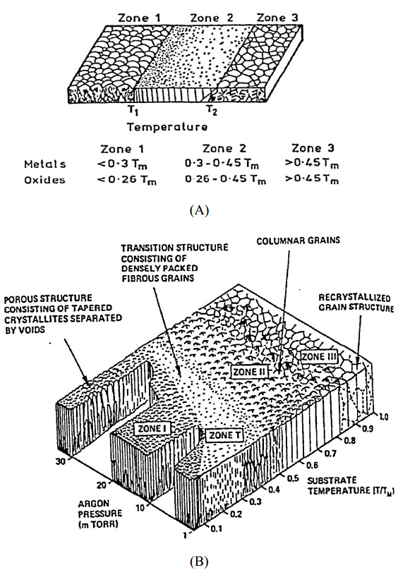
[105]	Movchan B, Demchishin A (1969) Structure and properties of thick condensates of nickel, titanium, tungsten, aluminum oxides, and zirconium dioxide in vacuum. Fiz Metal Metalloved 28: 653–660.
[106]	Thornton JA (1977) High rate thick film growth. Annu Rev Mater Sci 7: 239–260. doi: 10.1146/annurev.ms.07.080177.001323
[107]	Messier R, Giri A, Roy R (1984) Revised structure zone model for thin film physical structure. J Vac Sci Technol A 2: 500–503. doi: 10.1116/1.572604
[108]	Singh V (2004) Synthesis, structure, and tribological behavior of nanocomposite DLC based thin films [PhD thesis]. Louisiana State University.
[109]	Dresden-rossendorf I, Doctor G (2010) Growth, structure and magnetic properties of magnetron sputtered FePt thin films [PhD thesis]. Technische Universität Dresden.
[110]	Wang B, Fu X, Song S, et al. (2018) Simulation and Optimization of Film Thickness Uniformity in Physical Vapor Deposition. Coatings 8: 325. doi: 10.3390/coatings8090325
[111]	Divi S, Chatterjee A (2014) Study of Silicon Thin Film Growth at High Deposition Rates Using Parallel Replica Molecular Dynamics Simulations. Energy Procedia 54: 270–280. doi: 10.1016/j.egypro.2014.07.270
[112]	Allen MP (2004) Introduction to molecular dynamics simulation, In: Attig N, Binder K, Grubmuller H, Computational soft matter: from synthetic polymers to proteins, 23: 1–28.
[113]	Sutmann G (2002) Classical molecular dynamics and parallel computing, Germany: FZJ-ZAM-IB.
[114]	Rasoulian S, Ricardez-Sandoval LA (2015) Worst-case and distributional robustness analysis of a thin film deposition process. 9th International Symposium on Advanced Control of Chemical Processes, 7–10.
[115]	Li J, Croiset E, Ricardez-Sandoval L (2015) Carbon nanotube growth: First-principles-based kinetic Monte Carlo model. J Catal 326: 15–25. doi: 10.1016/j.jcat.2015.03.010
[116]	Family F (1986) Scaling of rough surfaces: effects of surface diffusion. J Phys A 19: 441. doi: 10.1088/0305-4470/19/8/006
[117]	Tang L, Nattermann T (1991) Kinetic roughening in molecular-beam epitaxy. Phys Rev Lett 66: 2899. doi: 10.1103/PhysRevLett.66.2899
[118]	Bhute VJ, Chatterjee A (2013) Building a kinetic Monte Carlo model with a chosen accuracy. J Chem Phys 138: 244112. doi: 10.1063/1.4812319
[119]	Bhute VJ, Chatterjee A (2013) Accuracy of a Markov state model generated by searching for basin escape pathways. J Chem Phys 138: 084103. doi: 10.1063/1.4792439
[120]	Lou Y, Christofides PD (2003) Estimation and control of surface roughness in thin film growth using kinetic Monte-Carlo models. Chem Eng Sci 58: 3115–3129. doi: 10.1016/S0009-2509(03)00166-0
[121]	Theodoropoulou A, Adomaitis RA, Zafiriou E (1998) Model reduction for optimization of rapid thermal chemical vapor deposition systems. IEEE T Semiconduct M 11: 85–98. doi: 10.1109/66.661288
[122]	Middlebrooks SA, Rawlings JB (2007) Model Predictive Control of Si_1−xGe_x Thin Film Chemical–Vapor Deposition. IEEE T Semiconduct M 20: 114–125. doi: 10.1109/TSM.2007.895203
[123]	Rasoulian S, Ricardez-Sandoval LA (2015) Robust multivariable estimation and control in an epitaxial thin film growth process under uncertainty. J Process Contr 34: 70–81. doi: 10.1016/j.jprocont.2015.07.002
[124]	Ricardez‐Sandoval LA (2011) Current challenges in the design and control of multiscale systems. Can J Chem Eng 89: 1324–1341. doi: 10.1002/cjce.20607
[125]	Vlachos DG (2005) A review of multiscale analysis: examples from systems biology, materials engineering, and other fluid–surface interacting systems. Adv Chem Eng 30: 1–61. doi: 10.1016/S0065-2377(05)30001-9
[126]	Chaffart D, Ricardez-Sandoval LA (2018) Optimization and control of a thin film growth process: A hybrid first principles/artificial neural network based multiscale modelling approach. Comput Chem Eng 119: 465–479. doi: 10.1016/j.compchemeng.2018.08.029
[127]	Jensen KF, Rodgers ST, Venkataramani R (1998) Multiscale modeling of thin film growth. Curr Opin Solid St M 3: 562–569. doi: 10.1016/S1359-0286(98)80026-0
[128]	Baumann F, Chopp D, De La Rubia TD, et al. (2001) Multiscale modeling of thin-film deposition: applications to Si device processing. MRS Bull 26: 182–189. doi: 10.1557/mrs2001.40
[129]	Zhang P, Zheng X, Wu S, et al. (2004) Kinetic Monte Carlo simulation of Cu thin film growth. Vacuum 72: 405–410. doi: 10.1016/j.vacuum.2003.08.013
[130]	Evans RD, Ricardez-Sandoval LA (2014) Multi-scenario modelling of uncertainty in stochastic chemical systems. J Comput Phys 273: 374–392. doi: 10.1016/j.jcp.2014.05.028
[131]	Chaffart D, Ricardez-Sandoval LA (2017) Robust dynamic optimization in heterogeneous multiscale catalytic flow reactors using polynomial chaos expansion. J Process Contr 60: 128–140. doi: 10.1016/j.jprocont.2017.07.002
[132]	Rasoulian S, Ricardez-Sandoval LA (2016) Stochastic nonlinear model predictive control applied to a thin film deposition process under uncertainty. Chem Eng Sci 140: 90–103. doi: 10.1016/j.ces.2015.10.004
[133]	Rasoulian S, Ricardez-Sandoval LA (2015) A robust nonlinear model predictive controller for a multiscale thin film deposition process. Chem Eng Sci 136: 38–49. doi: 10.1016/j.ces.2015.02.002
[134]	Allgöwer F, Findeisen R, Nagy ZK (2004) Nonlinear model predictive control: From theory to application. J Chin Inst Chem Engrs 35: 299–315.
[135]	Hu G, Orkoulas G, Christofides PD (2009) Modeling and control of film porosity in thin film deposition. Chem Eng Sci 64: 3668–3682. doi: 10.1016/j.ces.2009.05.008
[136]	Li C, Song S, Gibson D, et al. (2017) Modeling and validation of uniform large-area optical coating deposition on a rotating drum using microwave plasma reactive sputtering. Appl Optics 56: C65–C70. doi: 10.1364/AO.56.000C65
[137]	Heirung TAN, Paulson JA, O'Leary J, et al. (2018) Stochastic model predictive control-how does it work? Comput Chem Eng 114: 158–170. doi: 10.1016/j.compchemeng.2017.10.026
[138]	Koronaki E, Gkinis P, Beex L, et al. (2018) Classification of states and model order reduction of large scale Chemical Vapor Deposition processes with solution multiplicity. Comput Chem Eng 121: 148–157.
[139]	Divi S, Chatterjee A (2014) Study of Silicon Thin Film Growth at High Deposition Rates Using Parallel Replica Molecular Dynamics Simulations. Energy Procedia 54: 270–280. doi: 10.1016/j.egypro.2014.07.270

Reader Comments

your name:*

Email:*
© 2019 the Author(s), licensee AIMS Press. This is an open access article distributed under the terms of the Creative Commons Attribution License (http://creativecommons.org/licenses/by/4.0)