Citation: Mariya Aleksandrova. Spray deposition of piezoelectric polymer on plastic substrate for vibrational harvesting and force sensing applications[J]. AIMS Materials Science, 2018, 5(6): 1214-1222. doi: 10.3934/matersci.2018.6.1214
| [1] | Ionut Claudiu Roata, Catalin Croitoru, Alexandru Pascu, Elena Manuela Stanciu . Photocatalytic coatings via thermal spraying: a mini-review. AIMS Materials Science, 2019, 6(3): 335-353. doi: 10.3934/matersci.2019.3.335 |
| [2] | Ouassim Hamdi, Frej Mighri, Denis Rodrigue . Piezoelectric cellular polymer films: Fabrication, properties and applications. AIMS Materials Science, 2018, 5(5): 845-869. doi: 10.3934/matersci.2018.5.845 |
| [3] | Ruby Maria Syriac, A.B. Bhasi, Y.V.K.S Rao . A review on characteristics and recent advances in piezoelectric thermoset composites. AIMS Materials Science, 2020, 7(6): 772-787. doi: 10.3934/matersci.2020.6.772 |
| [4] | G. A. El-Awadi . Review of effective techniques for surface engineering material modification for a variety of applications. AIMS Materials Science, 2023, 10(4): 652-692. doi: 10.3934/matersci.2023037 |
| [5] | Muhamed Shajudheen V P, Saravana Kumar S, Senthil Kumar V, Uma Maheswari A, Sivakumar M, Sreedevi R Mohan . Enhancement of anticorrosion properties of stainless steel 304L using nanostructured ZnO thin films. AIMS Materials Science, 2018, 5(5): 932-944. doi: 10.3934/matersci.2018.5.932 |
| [6] | Hidayah Mohd Ali Piah, Mohd Warikh Abd Rashid, Umar Al-Amani Azlan, Maziati Akmal Mohd Hatta . Potassium sodium niobate (KNN) lead-free piezoceramics: A review of phase boundary engineering based on KNN materials. AIMS Materials Science, 2023, 10(5): 835-861. doi: 10.3934/matersci.2023045 |
| [7] | Alexandre Lavrov . Discrete-element model of electrophoretic deposition in systems with small Debye length: effective charge, lubrication force, characteristic scales, and early-stage transport. AIMS Materials Science, 2019, 6(6): 1213-1226. doi: 10.3934/matersci.2019.6.1213 |
| [8] | Timur Zinchenko, Ekaterina Pecherskaya, Dmitriy Artamonov . The properties study of transparent conductive oxides (TCO) of tin dioxide (ATO) doped by antimony obtained by spray pyrolysis. AIMS Materials Science, 2019, 6(2): 276-287. doi: 10.3934/matersci.2019.2.276 |
| [9] | Abbas Hodroj, Lionel Teulé-Gay, Michel Lahaye, Jean-Pierre Manaud, Angeline Poulon-Quintin . Nanocrystalline diamond coatings: Effects of time modulation bias enhanced HFCVD parameters. AIMS Materials Science, 2018, 5(3): 519-532. doi: 10.3934/matersci.2018.3.519 |
| [10] | Qinghua Qin . Applications of piezoelectric and biomedical metamaterials: A review. AIMS Materials Science, 2025, 12(3): 562-609. doi: 10.3934/matersci.2025025 |
In recent years, piezoelectric generators have been widely investigated for harvesting the kinetic energy from the ambient environment and convert it into electrical energy [1,2,3]. It has been demonstrated that the piezoelectric ceramics, such as lead-zirconium titanate (PZT), barium titanate (BaTiO3) and zinc oxide (ZnO) could be practically realized as a microelectronic and even nanoelectronic device, and the conversion efficiency could be still satisfying. Currently, many one-dimensional and two-dimensional inorganic piezoelectric nanostructures with wire, tube and branch type formations are studied to improve the yield of the miniaturized devices [4,5]. However, due to environmental issues and problems with high brittleness and poor biocompatibility, the efforts have been directed to find analogs to the piezoelectric oxide materials, mainly with polymeric [6]. One of the most studied piezoelectric polymers is polyvinylidene fluoride (PVDF) in β-phase for variety of sensing and energy harvesting applications [7,8,9]. One of its major advantages is the great durability at deformation—PVDF can stand high stress greater than 10 GPa without polymer chains damage and material degradation, because of high elasticity. It was found that high quality PVDF films could be deposited by spin coating, only if few micrometers or few hundred of nanometers thickness is required. Otherwise, the average roughness of the surface has been not satisfying. In addition, voids and other defects have occurred, making the piezoelectric element, involving such film inefficient [10]. That's why for nanosystems where thinner films are needed alternative approach for PVDF growing must be found. In this way, it is expected that the piezoelectric energy harvesting approach will be established as a reliable technology for making self-sufficient power supply for low consumable electronics, in particular flexible and stretchable electronics. For this purpose, the rest of the layers in the harvesting device must consist of suitable organic materials, as well. One of the most suitable techniques for polymer coatings deposition in this case is spray coating, due to the possibility for precise control of the temperature and aerosol/particles yield, leading to self-assembling of the polymer chains and resulting in smooth defectless films [11].
In this paper, piezoelectric polymer PVDF films were deposited by spray deposition on flexible substrate of polyethylene terephthalate (PET), coated with conductive polymer poly(3, 4-ethylenedioxythiophene) polystyrene sulfonate (PEDOT:PSS), serving as an electrode film. The effect of the deposition conditions on the microstructure and morphology of the PVDF coatings was investigated and the piezoelectric response of the system PEDOT:PSS/PVDF/Ag with single polymer/polymer interface was measured. It was found that PEDOT:PSS could serve as a suitable base for growing of uniform, well ordered layer and then piezoelectric voltage could be measured.
The PET substrate was cleaned by isopropyl alcohol in a ultrasonic cleaner for 180 s. PEDOT:PSS solution 3.0% in H2O, high-conductivity grade was spin coated on PET for producing film with thickness 120 nm, serving as a bottom contact. The samples were soft-baked at 50 ℃. PVDF granules were dissolved in methyl-ethyl-ketone (MEK) and the solution prepared was stirred 1 hour at 60 ℃, following by filtration. Solution for spraying was prepared with two different concentrations (10 wt% and 20 wt%). Each of them werepulverized simultaneously with the PEDOT:PSS coated PET sample's heating at different temperatures in the range 30–80 ℃. The rest of the spray deposition conditions were fixed—spraying pressure was set to 3.8 bars, the nozzle orifice diameter to 200 µm, temperature maintenance accuracy was 0.2 ℃. Top contacts of thermal evaporated silver films were configured through shadow mask. Their shape (rectangular with size ratio width:length = 3:1) and location on the PVDF surface (near the periphery of the substrate) were selected based on previous study, where it was found that such patterning provides the highest sensitivity [12]. Scanning electron microscopy was conducted by SEM microscope JEOL JSM-6390LV. Fourier transform infrared spectrum (FTIR) was recorded by Shimadzu spectrophotometer IRPrestige-21 in transmission mode to identify the molecular components and the typical bonds for piezoelectric phase. Films thickness and roughness profile was measured by Tencor Alpha Step 200 profiler. Vibrational tests were conducted by laboratory made stand and the generated electrical signals were monitored on oscilloscope DQ2042CN. The setup for testing is provided elsewhere [13]. The ready device is fixed to an elastic beam that performs the vibration with a certain amplitude and frequency. Using metallic wires, the electrical connection from the electrodes to the measurement equipment is set, using silver paste. The vibration frequency was 50 Hz for all measurements, but the input voltage of the electromechanical system varied from 1 V, 3 V and 5 V, where 1 V corresponded to 25 N = 2.65 g, 3 V = 29 N = 2.95 g; 5 V = 34 N = 3.45 g.
The total eight combinations of devices with PEDOT:PSS/PVDF layers were examined by SEM with a magnification of 10000 times and compared in Figure 1. As can be seen from the microscopic images, the PVDF layer produced from 10 wt% spray deposited at 30 ℃ is non-uniform, because the solvent evaporation rate is very low. This is due to the relatively low temperature during spraying, which in turn causes the layer to leak. The layer lacks density and at 50 ℃ was still irregular. By increasing the temperature to 70 ℃, an improvement in the layer morphology was noted, with increased flatness and uniformity.
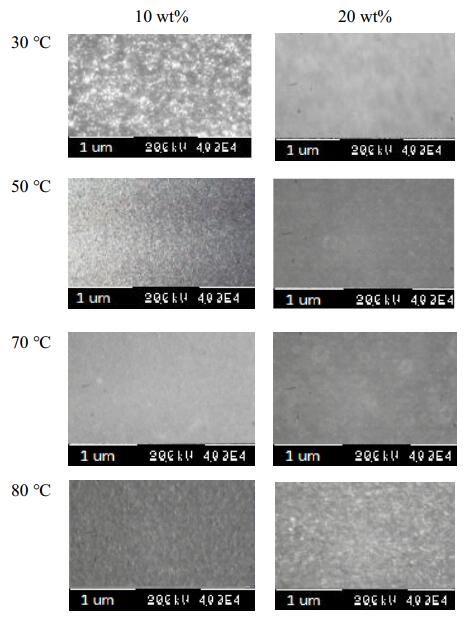 Figure 1. SEM images of the PVDF films produced by spray deposition on PET/PEDOT:PSS surface at different solution concentrations and different substrate temperatures.
At 80 ℃, dust-like particles were observed on the substrate as a result of the very strong heat field above the PEDOT:PSS, which causes the solvent molecules to be removed quickly, before the aerosols to reach the substrate. At PVDF solution with concentration of 20 wt% higher uniformity and smoother layers were observed at lower temperatures (50 ℃) compared to 10 wt% PVDF. When spraying at temperatures of 80 ℃, it was noted that the PVDF layer is irregular with a high average roughness. On the next substrates, the PVDF layers were deposited at the optimized temperatures—at 10 wt% PVDF solution the optimal temperature of 70 ℃ was used and at 20 wt% PVDF solution the optimum was 50 ℃. These combinations of deposition conditions produced sufficiently uniform layers to form large contact area with the electrodes to be applied thereto. As a result, it is expected a uniform polarization reaction and stable piezoelectric response of the polymer. Therefore, they were used for further analyses.
Regarding the presence of the typical piezoelectric β-phase in the PVDF polymer, FTIR analysis was conducted (Figure 2). For the sample prepared at 10 wt%, it was found that the spectrum very well coincides with the data available in the literature [14,15,16]. The characteristic absorption bands at wavenumbers 510–520,620–625,880–900, 1090, 1240, 1444, 1695 cm−1 presented and their intensity determined 72% piezoelectric phase. The rest of the bands in Figure 2 are related to α- and γ-PVDF phases, as well as some weak signal are generated due to PEDOT:PSS substrate. Some multiple overlapping bands in close range of few cm−1 are caused from impurities introduction due to the vacuum-free deposition process. For comparison, the highest reported content of β-phase in commercially available devices using PVDF is between 75% and 85% at thicker films in the micrometer range [17]. For the sample spray deposited from 20 wt% PDVF solution there was great dissipation of IR beam due to the higher roughness of the surface, which hinder the precise sweep of the transmitted bands as a function of the wavenumber. Nevertheless, we think that the results from FTIR are similar, because the voltage generated is with the same order of magnitude and close in value to the previous sample.
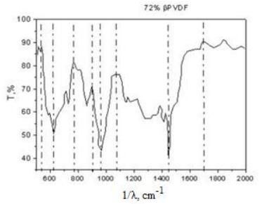 Figure 2. FTIR spectrum of PVDF on PET/PEDOT:PSS substrate spray deposited from 10 wt% solution.
The recorded profiles of both films surfaces (Figure 3) showed PVDF film thicknesses of 186 nm and 220 nm, respectively produced from 10 wt% and 20 wt% solution concentration. The corresponding average roughness was approximately 12 nm and 25 nm across the sample length of 1 cm, which is evidence for excellent uniformity.
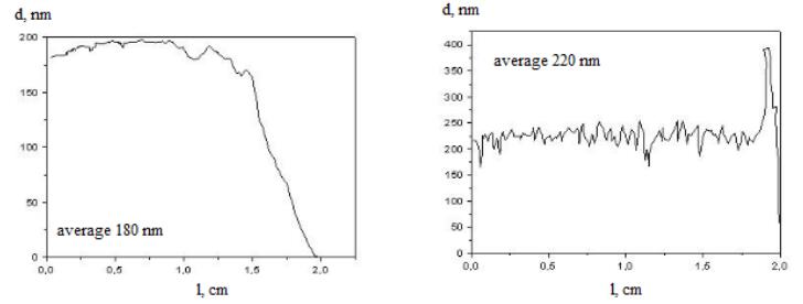 Figure 3. Profillograms of layers with different concentrations of PVDF—left: 10 wt%; right: 20 wt%.
After silver contacts deposition electrical characteristics in dynamic mode for both optimal cases (10 wt%, 70 ℃ and 20 wt%, 50 ℃) are measured in case of energy harvesting application. Figure 4 shows the output voltages of the two microelements. At the sample with 10 wt% PVDF layer and 25 N input vibrations, oscillations in the output voltage were observed, probably due to the lower content of piezoelectric polymer in the layer. Increasing the input vibrations' amplitude the generated voltage increased, but the distortions in its shape also increased. If a comparison is made with the signals generated under the same input conditions, but from the sample obtained at 20 wt%, 50 ℃, it can be seen that the voltage is more stable, with a more clearly defined shape, probably because of the higher density of the layers and higher piezoelectric active polymer content. However, it has lower amplitude for each of the input stimuli. As was detected by the profiler, the surface of the sensor obtained at 20 wt% and 50 ℃ showed higher roughness, which is probably the reason for more unstable electrical contact with the electrode and loss of energy (voltage drop) at the polymer/conductive polymer interface. This could explain smaller amplitude of the generated piezoelectric voltage despite the higher concentration of PVDF. Concrete values for the amplitude of the generated piezoelectric voltage at different supplied dynamic load can be seen under each oscillogram in Figure 4.
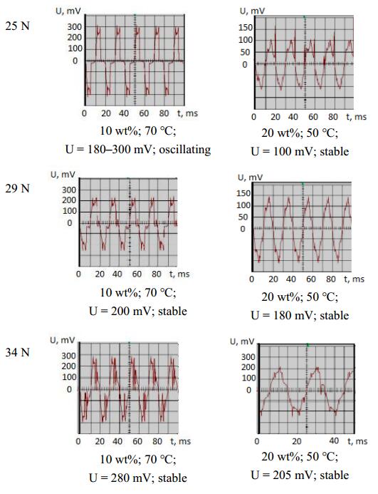 Figure 4. Generated piezoelectric voltage at supplied vibrations with different intensity on samples fabricated at the optimal conditions for spray deposition of both PVDF solutions.
The device can perform dual functions, serving as a force (or pressure) sensor too. The dependence of the generated voltage on the applied force in static mode is shown in Figure 5b (photo of the prepared sample is shown in Figure 5a), from where the linearity of the sensor in certain force range can be determined. The mean deviation from the ideal linear response for the sample obtained at 10 wt% PVDF is 48 mV, corresponding to 4.70% non-linearity (or linearity of 95.3%). For the sample obtained at 20 wt% PVDF this value is 44.6 mV, which corresponds to non-linearity of 3.72%. Voltage was registered when the weight is released from the sample and not when applied to it, which probably means that the element is better suited for working as a tension sensor rather than to compression.
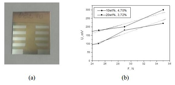 Figure 5. (a) Photo of the fabricated sample; (b) linearity of the polymeric piezoelectric devices, working like force sensors.
The polymer layer sensor exhibited a wider dynamic range, as compared with the PZT based sensor with similar constructive design and films thicknesses [12]. The piezoelectric response strength is comparable. At the same time, spraying technology is simpler, cheaper and faster to apply. In order to estimate the reliability of the structures with the enhanced electrical behavior (10 wt% of PVDF), they were subjected to a large number of vibration cycles. The set cycles were 6000, determined on the basis of the vibration period (the frequency of the input voltage of the electromechanical system) and the duration of vibrating. The goal was to determine the degree of degradation or sensitivity of the PEDOT:PSS/PVDF interface against repeating mechanical load. The output voltages were then measured again and it was found that there was a decrease in the amplitude reflected in Table 1. The results show excellent stability of the structures, which may ascribe to the closer Young modulus and high elasticity of both polymeric layers—piezoelectric and electrode.
| Parameters of the sample | Case 1 | Case 2 | Case 3 |
| Mechanical load, N | 25 | 29 | 34 |
| Uo, mV | 180 | 200 | 300 |
| U6000, mV | 172 | 180 | 250 |
| Relative deviation, % | 4.4 | 10 | 17 |
 DownLoad: CSV
Piezoelectric structures working as both energy harvesting and force sensors have been successfully obtained by spray deposition of PVDF on flexible substrate coated with conductive polymer. The results show that for specific solution concentration (PVDF 10 wt%) if heating the substrate at 70 ℃ smooth, uniform thin film with good adhesion on the conductive polymer coating and high content of piezoelectric phase could be obtained. As a result, energy harvesting device with small non-linear distortions of the signal and force sensor with high linearity can be fabricated. The PEDOT:PSS/PVDF interface demonstrated significant mechanical durability at multiple bending, making this technology and design approach preferable for flexible and stretchable electronics.
The work is funded by BNSF, grant No DH 07/13. The author is thankful to Prof. Kostadinka Gesheva from CL-SENES, BAS for the measured FTIR spectrum and Dr. Georgi Kolev from TU-Sofia for the PVDF material provided.
The author declares no conflict of interest.
| [1] | Chen J, Oh SK, Zou H, et al. (2018) High-output lead-free flexible piezoelectric generator using single-crystalline GaN thin film. ACS Appl Mater Inter 18: 12839–12846. |
| [2] |
Walubita LF, Djebou DCS, Faruk ANM, et al. (2018) Prospective of societal and environmental benefits of piezoelectric technology in road energy harvesting. Sustainability 10: 383–396. doi: 10.3390/su10020383

|
| [3] |
Rocha JG, Goncalves LM, Rocha PF, et al. (2010) Energy harvesting from piezoelectric materials fully integrated in footwear. IEEE T Ind Electron 57: 813–819. doi: 10.1109/TIE.2009.2028360
|
| [4] |
Johar AM, Hassan MA, Waseem A, et al. (2018) Stable and high piezoelectric output of GaN nanowire-based lead-free piezoelectric nanogenerator by suppression of internal screening. Nanomaterials 8: 437–449. doi: 10.3390/nano8060437
|
| [5] |
Yan J, Jeong YG (2017) Roles of carbon nanotube and BaTiO3 nanofiber in the electrical, dielectric and piezoelectric properties of flexible nanocomposite generators. Compos Sci Technol 144: 1–10. doi: 10.1016/j.compscitech.2017.03.015
|
| [6] |
Jung I, Shin YH, Kim S, et al. (2017) Flexible piezoelectric polymer-based energy harvesting system for roadway applications. Appl Energ 197: 222–229. doi: 10.1016/j.apenergy.2017.04.020
|
| [7] |
Ghafari E, Jiang XD, Lu N (2018) Surface morphology and beta-phase formation of single polyvinylidene fluoride (PVDF) composite nanofibers. Adv Compos Hybrid Mater 1: 332–340. doi: 10.1007/s42114-017-0016-z
|
| [8] |
Ghafari E, Lu N (2019) Self-polarized electrospun polyvinylidene fluoride (PVDF) nanofiber for sensing applications. Compos Part B-Eng 160: 1–9. doi: 10.1016/j.compositesb.2018.10.011
|
| [9] |
Su YF, Kotian RR, Lu N (2018) Energy harvesting potential of bendable concrete using polymer based piezoelectric generator. Compos Part B-Eng 153: 124–129. doi: 10.1016/j.compositesb.2018.07.018
|
| [10] |
Zhu Z, Lowes J, Berron J, et al. (2014) Spin-coating defect theory and experiments. ECS Trans 60: 293–302. doi: 10.1149/06001.0293ecst
|
| [11] | Xu Y, Luo A, Zhang A, et al. (2016) Spray coating of polymer electret with nano particles for stable surface charge. IEEE 11th Annual International Conference on Nano/Micro Engineered and Molecular Systems (NEMS), 17–20 April 2016, Sendai, Japan. |
| [12] | Kolev G, Aleksandrova M, Videkov V, et al. (2012) Piezoelectric MEMS stress sensor with thin lead zirconate titanate (PZT) layer. IEEE 20th Telecommunications Forum (TELFOR), Belgrade, Serbia, 991–993. |
| [13] |
Aleksandrova M, Kurtev N, Videkov V, et al. (2015) Material alternative to ITO for transparent conductive electrode in flexible display and photovoltaic devices. Microelectron Eng 145: 112–116. doi: 10.1016/j.mee.2015.03.053
|
| [14] | Thirmal C, Nayek C, Murugavel P, et al. (2013) Magnetic, dielectric and magnetodielectric properties of PVDF-La0.7Sr0.3MnO3 polymer nanocomposite film. AIP Adv 3: 112109. |
| [15] |
Ruan L, Yao X, Chang Y, et al. (2018) Properties and applications of the β phase poly(vinylidene fluoride). Polymers 10: 228–255. doi: 10.3390/polym10030228
|
| [16] | Mandal D, Henkel K, Schmeißer D (2011) Control of the crystalline polymorph, molecular dipole and chain orientations in P(VDF-HFP) for high electrical energy storage application. 2011 International Conference on Nanoscience, Technology and Societal Implications (NSTSI), Bhubaneswar, India. |
| [17] | Parker A, Ueda A, Marvinney CE, et al. (2018) Structural and thermal treatment evaluation of electrospun PVDF nanofibers for sensors. J Polym Sci Appl 2: 1–4. |
| 1. | I Kralov, K Nedelchev, Lowering the noise level in the transport flows through reduction of the traffic barrier reflected noise, 2019, 618, 1757-899X, 012051, 10.1088/1757-899X/618/1/012051 | |
| 2. | Sakti Prasanna Muduli, S Parida, S K Rout, Shailendra Rajput, Manoranjan Kar, Effect of hot press temperature on β-phase, dielectric and ferroelectric properties of solvent casted Poly(vinyledene fluoride) films, 2019, 6, 2053-1591, 095306, 10.1088/2053-1591/ab2d85 | |
| 3. | A A Pan’kov, Indicator polymer coating with built-in fiber optic piezosensor, 2021, 1029, 1757-899X, 012072, 10.1088/1757-899X/1029/1/012072 | |
| 4. | G. Hassnain Jaffari, M. Shahid Iqbal Khan, Fiza Mumtaz, Y. Wang, Nawazish Ali Khan, Manipulation of crystallization and dielectric relaxation dynamics via hot pressing and copolymerization of PVDF with Hexafluoropropylene, 2023, 30, 1022-9760, 10.1007/s10965-022-03395-7 | |
| 5. | Rukhsar Ali Khan, Munir Ashraf, Amjed Javid, Kashif Iqbal, Abher Rasheed, Nadeem Nasir, Development of self-polarized PVDF films on carbon fabrics for sensing applications, 2022, 113, 0040-5000, 2208, 10.1080/00405000.2021.1974687 | |
| 6. | Sepide Taleb, Miguel A. Badillo-Ávila, Mónica Acuautla, Fabrication of poly (vinylidene fluoride) films by ultrasonic spray coating; uniformity and piezoelectric properties, 2021, 212, 02641275, 110273, 10.1016/j.matdes.2021.110273 | |
| 7. | Rostislav P. Rusev, 2023, Piezo Effect of Polyvinylidene Fluoride Layer with Rochelle Salt, 979-8-3503-0200-4, 1, 10.1109/ET59121.2023.10278991 | |
| 8. | Mariya Aleksandrova, Tsvetozar Tsanev, Berek Kadikoff, Dimiter Alexandrov, Krasimir Nedelchev, Ivan Kralov, Piezoelectric Elements with PVDF–TrFE/MWCNT-Aligned Composite Nanowires for Energy Harvesting Applications, 2023, 13, 2073-4352, 1626, 10.3390/cryst13121626 |


Figures(5) / Tables(1)

Mariya Aleksandrova. Spray deposition of piezoelectric polymer on plastic substrate for vibrational harvesting and force sensing applications[J]. AIMS Materials Science, 2018, 5(6): 1214-1222. doi: 10.3934/matersci.2018.6.1214

| Parameters of the sample | Case 1 | Case 2 | Case 3 |
| Mechanical load, N | 25 | 29 | 34 |
| Uo, mV | 180 | 200 | 300 |
| U6000, mV | 172 | 180 | 250 |
| Relative deviation, % | 4.4 | 10 | 17 |
DownLoad: CSV


