


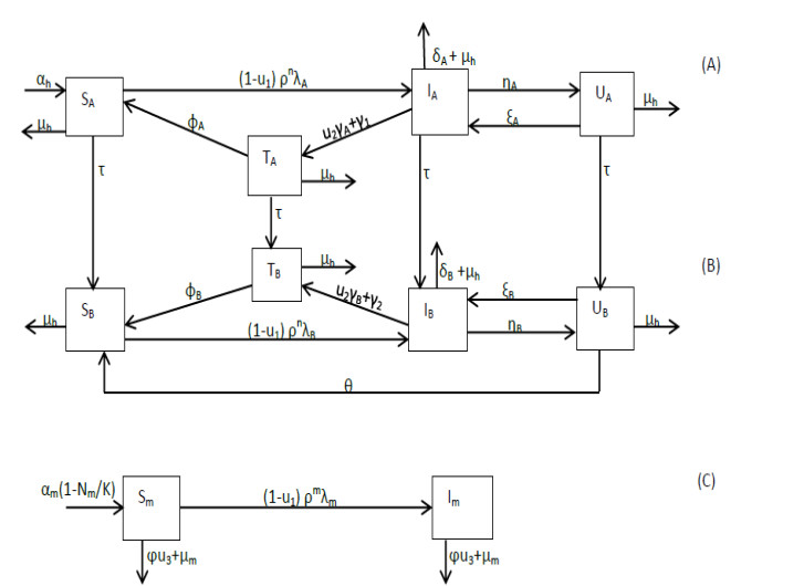
Figure 1.
Schematic diagram of malaria transmission: (A) infants – humans five years old and younger, (B) adults – humans older than 5 years and (C) female Anopheles mosquitoes.
Citation: Tabinda Sattar, Muhammad Athar. Nano bio-MOFs: Showing drugs storage property among their multifunctional properties[J]. AIMS Materials Science, 2018, 5(3): 508-518. doi: 10.3934/matersci.2018.3.508
| [1] | Thomas C. Chiang . Economic policy uncertainty and stock returns—evidence from the Japanese market. Quantitative Finance and Economics, 2020, 4(3): 430-458. doi: 10.3934/QFE.2020020 |
| [2] | Saeed Sazzad Jeris, Ridoy Deb Nath . Covid-19, oil price and UK economic policy uncertainty: evidence from the ARDL approach. Quantitative Finance and Economics, 2020, 4(3): 503-514. doi: 10.3934/QFE.2020023 |
| [3] | Sudeshna Ghosh . Asymmetric impact of COVID-19 induced uncertainty on inbound Chinese tourists in Australia: insights from nonlinear ARDL model. Quantitative Finance and Economics, 2020, 4(2): 343-364. doi: 10.3934/QFE.2020016 |
| [4] | Md Akther Uddin, Mohammad Enamul Hoque, Md Hakim Ali . International economic policy uncertainty and stock market returns of Bangladesh: evidence from linear and nonlinear model. Quantitative Finance and Economics, 2020, 4(2): 236-251. doi: 10.3934/QFE.2020011 |
| [5] | Gülserim Özcan . The amplification of the New Keynesian models and robust optimal monetary policy. Quantitative Finance and Economics, 2020, 4(1): 36-65. doi: 10.3934/QFE.2020003 |
| [6] | Diogo Matos, Luís Pacheco, Júlio Lobão . Availability heuristic and reversals following large stock price changes: evidence from the FTSE 100. Quantitative Finance and Economics, 2022, 6(1): 54-82. doi: 10.3934/QFE.2022003 |
| [7] | Simiso Msomi, Damien Kunjal . Industry-specific effects of economic policy uncertainty on stock market volatility: A GARCH-MIDAS approach. Quantitative Finance and Economics, 2024, 8(3): 532-545. doi: 10.3934/QFE.2024020 |
| [8] | Chiao Yi Chang, Fu Shuen Shie, Shu Ling Yang . The relationship between herding behavior and firm size before and after the elimination of short-sale price restrictions. Quantitative Finance and Economics, 2019, 3(3): 526-549. doi: 10.3934/QFE.2019.3.526 |
| [9] | Serçin ŞAHİN, Serkan ÇİÇEK . Interest rate pass-through in Turkey during the period of unconventional interest rate corridor. Quantitative Finance and Economics, 2018, 2(4): 837-859. doi: 10.3934/QFE.2018.4.837 |
| [10] | Albert A. Agyemang-Badu, Fernando Gallardo Olmedo, José María Mella Márquez . Conditional macroeconomic and stock market volatility under regime switching: Empirical evidence from Africa. Quantitative Finance and Economics, 2024, 8(2): 255-285. doi: 10.3934/QFE.2024010 |
Malaria, although preventable and treatable, continues to be one of the most prevalent and lethal human infections worldwide [1]. Globally, 627,000 deaths were recorded in 2020, with Sub-Saharan Africa accounting for almost 96% of them [2]. Children under 5 years become the most vulnerable to infection and death after losing their maternal antibodies, which protect them during their first six months [3,4].
A massive deployment of effective prevention and treatment tools by the World Health Organization (WHO) in 2000 has led to a reduction of cases in the Americas and the Western Pacific Region, no indigenous cases in the European Region, a decline of 66% in all age mortality rates in Africa and 663 million cases being averted in Sub-Saharan Africa from 2001 to 2015 [5,6]. During this period, it is estimated that Sub-Saharan Africa saved USfanxiexian_myfh900 million in case management costs. In 2019, the governments of the endemic countries and their international partners invested funding estimated at USfanxiexian_myfh 3.0 billion for malaria control and elimination [2].
Early treatment of infected humans with effective antimalarial drugs gives complete recovery and prevents the transmission of infection to mosquitoes during a blood meal, recrudescence, severe malaria and even death [7]. Recrudescence is common in Plasmodium falciparum infection and may occur when parasites, which remain in the red blood cells after an episode of malaria, start multiplying and cause the recurrence of the clinical symptoms due to treatment failure in the patient [8]. P. falciparum is the most deadly species of malaria parasite globally and the most prevalent in Africa. In most Sub-Saharan countries, after P. falciparum resistance was identified, the treatment for uncomplicated malaria was changed to artemisinin-based combination therapy (ACT) [7,9]. WHO recommends that an entire course of highly effective ACT must be used by both semi-immune and non-immune malaria patients to have a complete cure from both sexual and asexual forms of the parasites and partial immunity [5,7].
The availability, distribution, trade and use of monotherapies and other substandard antimalarial drugs continue throughout most malaria-endemic countries [10,11,12,13,14,15,16]. It is estimated that about a third of antimalarial drugs that end up in Africa are counterfeit [13,15]. These antimalarial drugs may contain too few or too many required active ingredients and may fail to be adequately absorbed by the body [17]. Recently, evidence has shown that counterfeit antimalarial drugs pose a public health threat of prolonging the illness, incomplete recovery, treatment failure, recrudescence, severe disease, spreading drug resistance and asymptomatic infection carriers, resulting in more than 122,000 deaths of African children under five years annually [7,12,15,17,18]. According to [4,13], the use of these drugs may jeopardize the success made so far in controlling and eliminating malaria, particularly in Sub-Saharan Africa.
Several mathematical models have considered the effects of effective treatment [19,20,21,22,23], recovery or immunity [19,24,25,26,27,28], reinfection [27,29,30] and age-structure [21,22,31,32] on the dynamics of malaria. In particular, [19,24,25,26,27,28,33] incorporated into their models recovered or semi-immune humans, who are reservoirs of infection to mosquitoes. In addition, [27] assumed that the recovered humans could relapse. Evidence has shown that in most malaria-endemic areas in Sub-Saharan Africa, symptomatic humans often use counterfeit and effective drugs for treatment [4,9,11,12,13,14,15,16]. The aforementioned models did not consider the effect of both effective and counterfeit antimalarial drugs on the dynamics of malaria.
Many studies have also been carried out to examine the impact of control strategies on the transmission of malaria infection. The potential impact of personal protection, treatment and possible vaccination on the transmission dynamics of malaria was theoretically assessed in [20]. The optimal control theory has been successfully used in decisions concerning the cost minimization of several control intervention models after implementing Pontryagin's maximum principle [34]. The studies [23,24,35,36,37,38] applied optimal control theory to determine the impact of control strategies on the transmission dynamics of malaria. The studies investigated optimal strategies for controlling the spread of malaria disease using treatment, treated bednets and spraying of mosquito insecticide in models with mass action [24], standard [23,37] or non-linear [36] incidence rates and cost-effectiveness [23] of the controls. Other studies [38] used optimal control problem strategies to study how genetically modified mosquitoes should be introduced into the environment. The aforementioned studies did not consider optimal control in age-structured models, especially where the treatment can be either effective or ineffective due to using effective or counterfeit antimalarial drugs. Optimal control has, however, been applied to an age-structured model for HIV [39].
This paper seeks to answer the following question: What optimal control strategy best eliminates P. falciparum malaria infection in an age-structured population where counterfeit drug use persists? We do this by developing a deterministic model for malaria transmission incorporating the infant and adult populations, counterfeit drug use and three of the malaria control measures adopted by most endemic countries in Sub-Saharan Africa [4,40], namely, use of highly effective antimalarial drugs (HEAs), insecticide-treated bednets (ITNs) and indoor residual spraying (IRS). The paper is organized as follows. Section 2 briefly describes the formulation of the model and its basic properties. In Section 3, the dynamics of the model is presented. The analysis of the reproduction number is done in Section 4. In Section 5, the analysis of the optimal control problem is undertaken to find the conditions for optimal malaria control using Pontryagin's maximum principle, and the numerical simulations of the model are illustrated. The discussion of results and conclusion are presented in Sections 6 and 7, respectively.
The transmission model for malaria in human and female anopheles mosquito populations is formulated with the total population sizes at time t given by Nh(t) and Nm(t), respectively. The human population is divided into two mutually exclusive age subgroups: infants aged 0–5 years and adults above five. Each age subgroup is divided into susceptible, infectious, counterfeit antimalarial drug users and effective antimalarial drug users epidemiological classes. The mosquito population is divided into susceptible and infectious epidemiological classes. Figure 1 shows the flows between the classes. We let SA(SB), IA(IB), UA(UB) and TA(TB) represent infants (adults) who are susceptible, infectious, counterfeit drug users and effective drug users, respectively. For the mosquito population, Sm and Im denote the susceptibles and infectives, respectively. The total human population Nh(t) at a time t is given by
| Nh(t)=NA(t)+NB(t)=SA(t)+IA(t)+UA(t)+TA(t)+SB(t)+IB(t)+UB(t)+TB(t). |
The total mosquito population Nm(t) at a given time t is given by Nm(t) = Sm(t)+Im(t).
Susceptible humans are those with no merozoites or gametocytes in their bodies. Infectious humans show clinical symptoms of malaria and can infect feeding mosquitoes. Users of effective antimalarial drugs recover from malaria either naturally or due to using an effective antimalarial drug. These humans have partial immunity and become susceptible when this immunity wanes. Counterfeit drug users are humans who are removed from the infectious class due to using counterfeit drugs to treat malaria. They are asymptomatic, can infect mosquitoes (at a lower rate compared to the infectious humans) and can recrudesce into the infectious class. Adult counterfeit drug users can become susceptible due to the high level of acquired immunity resulting from their repeated exposures to malaria [3]. The susceptible mosquitoes have no sporozoites in their body. Infective mosquitoes can infect humans during a blood meal. It is assumed that the infective stage of the mosquitoes ends with their death due to their short life cycle. Merozoites are the parasites released into the human bloodstream when a hepatic or erythrocytic schizont bursts, and gametocytes are the sexual stages of malaria parasites that infect anopheline mosquitoes when taken up during a blood meal. On the other hand, sporozoites are the motile malaria parasites inoculated by feeding female anopheline mosquitoes to invade the human hepatocytes [7].
The susceptible infants class, SA, is generated by the recruitment of newborns at a birth rate αh and the loss of post-treatment prophylaxis by effectively treated infants at a per capita rate ϕA. This class is decreased when infants in it die naturally, mature into susceptible adults or get infected, at a per capita natural death rate μh, per capita rate τ of maturing and per capita infection rate of infants (1−u1)ρnλA, respectively. The control u1 represents the effort of preventing malaria with insecticide-treated bednets (ITNs), so (1−u1) describes the failure probability of this prevention effort. The daily survival probability of a human is assumed to be ρ1=e−μh. The probability of survival of a human over the average latent period of length nh to be infectious is given by ρn=e−μhnh. λA is the force of infection in infants.
The infectious infants class, IA, is generated by the per capita rate of acquiring infection (1−u1)ρnλA and per capita recrudescence rate, ξA, of infants who used counterfeit drugs. This class is reduced by the per capita natural death rate μh, per capita disease-induced death rate δA, per capita removal rate due to the use of counterfeit drugs ηA, per capita recovery rate due to the use of a highly effective antimalarial and natural recovery u2γA+γ1, and per capita rate of maturing into infectious adults τ of infants in it. The control u2 represents the treatment efforts with highly effective antimalarials and involves diagnosing patients, administering drug intake and follow-up of drug management. The recovery rate in infants due to using a highly effective antimalarial drug is γA, and γ1 is the natural recovery rate in infants.
The infant class of counterfeit drug users, UA, increases at a per capita removal rate ηA of infectious infants due to counterfeit drug use and decreases at a per capita recrudescence rate ξA into infectious infants, per capita natural death rate μh and per capita rate of maturing into adults τ of infants who used counterfeit malaria drugs.
The infant class of effective drug users, TA, increases with the per capita recovery rate u2γA+γ1 of infectious infants. This class decreases due to the loss of post-treatment prophylaxis at a per capita rate ϕA, natural death at a per capita natural death rate μh and maturing into adults at a per capita rate τ of infants in it.
The susceptible adults class, SB, is generated when the susceptible infants mature above 5 years, recovered adults lose their partial immunity and post-treatment prophylaxis at a per capita rate ϕB, and counterfeit drug users become susceptible at a per capita rate θ. This class is decreased by natural death and infections, with, respectively, per capita natural death rate μh and per capita rate of acquiring infection from infectious mosquitoes (1−u1)ρnλB, where λB is the force of infection in adults.
The infectious adults class, IB, increases when infectious infants mature above 5 years, and adults recrudesce at per capita rate ξB and acquire infection at rate (1−u1)ρnλB. The class is reduced at per capita natural death rate μh, per capita disease-induced death rate δB, per capita removal rate ηB due to counterfeit drugs use and recovery at per capita rate u2γB+γ2 of adults in it. The recovery rate of adults due to using an effective malarial drug is γB, and γ2 is the natural recovery rate of adults.
The adult class of counterfeit drug users, UB, increases when infants who used counterfeit drugs mature above 5 years and when the infectious adults who used counterfeit drugs are removed at a per capita rate ηB. This class decreases by natural death, recrudescence and reverting to the susceptible class of adults in it, with, respectively, per capita natural death rate μh, recrudescence rate ξB and susceptibility of adults θ.
The adult class of effective drug users, TB, increases when infants in the infant class of effective drug users mature above 5 years and when the infectious adults recover at a per capita rate u2γB+γ2. This class decreases by natural death, loss of immunity and post-treatment prophylaxis of adults with, respectively, per capita natural death rate μh and per capita loss of partial immunity and post-treatment prophylaxis rate ϕB.
Susceptible female Anopheles mosquitoes are recruited at a per capita rate αm(1−NmK), where αm is the birth rate of mosquitoes, and K is the environmental carrying capacity of pupa [41]. They die at a per capita natural death rate μm and a per capita indoor residual spraying (IRS) induced death rate φu3. The control u3 represents the prevention effort with the IRS and includes spraying with insecticide and surveillance. φ is the proportion of mortality induced by IRS. We assume that the mosquito population does not go extinct, and hence rm = αm−μm−φu3>0. Most of the analysis is redundant if rm<0. The mosquitoes become infected by humans in the infectious and counterfeit drug users class at a rate (1−u1)ρmλm, where λm is the force of infection rate in mosquitoes. The daily survival probability of a mosquito is assumed to be ρ2=e−μm. The probability of survival of a mosquito over the average latent period of length nm and becoming infectious is given by ρm=e−μmnm.
The infective mosquito population increases when mosquitoes acquire infection from humans at a per capita rate (1−u1)ρmλm. It decreases with a per capita natural death rate μm and a per capita IRS-induced death rate φu3.
Differences have been observed in malaria transmission rates, degree of infectivity, recovery and immunity due to strains, exposure, locality, age and treatment [3,4,7,42,43]. In humans, the gametocyte rate and density [42], as well as the parasite rate [42,44], have been found to decrease with age. Thus, we assume that infants have higher infectiousness to mosquitoes than adults. The degree of infectivity in the human population is denoted by the parameter πi,i=1,2,3, where π1,π2 and π3 are associated, respectively, with IB,UA and UB such that 0<π3<π2<π1<1. Further, the transmission probabilities in infants, adults and mosquitoes are denoted by βA, βB and βm, respectively. The average numbers of mosquito bites per infant and adult per time unit are denoted by a and b, respectively, and c is the average number of bites given by a mosquito per time unit.
Usually, the recruitment of children is dependent on the adult population. At the same time, the children mature and move to the adult population. If the population of adults is much larger than that of children, we can assume that it is constant and not affected by the latter. In this case, the total birth rate αh is just the per capita birth rate in the adult population αB multiplied by NB, αh=αBNB.
The above formulations and assumptions give the following system of ordinary differential equations for the structured malaria model:
| dSAdt=αh+ϕATA−(e−μhnh(1−u1)λA+τ+μh)SA, | (2.1) |
| dSBdt=τSA+ϕBTB+θUB−(e−μhnh(1−u1)λB+μh)SB, | (2.2) |
| dIAdt=e−μhnh(1−u1)λASA+ξAUA−d1IA, | (2.3) |
| dIBdt=τIA+e−μhnh(1−u1)λBSB+ξBUB−d2IB, | (2.4) |
| dUAdt=ηAIA−d3UA, | (2.5) |
| dUBdt=τUA+ηBIB−d4UB, | (2.6) |
| dTAdt=(u2γA+γ1)IA−(ϕA+τ+μh)TA, | (2.7) |
| dTBdt=τTA+(u2γB+γ2)IB−(ϕB+μh)TB, | (2.8) |
| dSmdt=αm(1−NmK)Nm−(e−μmnm(1−u1)λm+μm+φu3)Sm, | (2.9) |
| dImdt=e−μmnm(1−u1)λmSm−(μm+φu3)Im, | (2.10) |
with initial conditions
| SA(0)>0,SB(0)>0,IA(0)≥0,IB(0)≥0,UA(0)≥0,UB(0)≥0,TA(0)≥0,TB(0)≥0,Sm(0)>0,Im(0)≥0, |
where
| λA=aβANhIm,λB=bβBNhIm,λm=cβmNh(IA+π1IB+π2UA+π3UB), |
| d1=δA+ηA+u2γA+γ1+τ+μh,d2=δB+ηB+u2γB+γ2+μh,d3=ξA+τ+μhandd4=ξB+θ+μh. |
The parameter values of the malaria control model are shown in Table 1 in Section 5. The age-structured models (2.1)–(2.10) is an extension of the malaria model developed in [45], by including differentiated susceptibility, infectivity and infectiousness of infant and adult populations and control measures to malaria.
| Parameter | Value/Range | Unit | References | Parameter | Value/Range | Unit | References |
| αh | 0.3002 | day−1 | Estimated | π1 | 0.5/[0, 1] | Assumed | |
| αm | 0.2 | day−1 | Estimated | π2 | 0.2/[0, 1] | Assumed | |
| τ | 15×365 | day−1 | Estimated | π3 | 0.1/[0, 1] | Assumed | |
| a | 11/[1,2,3,4,5,6,7,8,9,10,11,12,13,14,15,16,17,18,19,20,21,22,23,24,25,26,27,28,29,30,31,32,33,34] | day−1 | [52,53,54,55] | ηA | [17-130] | day−1 | [7,9,48] |
| b | 5/[1,2,3,4,5,6,7,8,9,10,11,12,13,14,15,16,17,18,19,20,21,22,23,24,25,26,27,28,29,30,31,32,33,34] | day−1 | [52,53,54,55] | ηB | [17-130] | day−1 | [7] |
| c | 3 | day−1 | [35] | γA | 14/[13-130] | day−1 | [7,9] |
| βA | 0.0005 | Estimated | γB | 14/[13-130] | day−1 | [7] | |
| βB | 0.0005 | Estimated | ξA | [17-130] | day−1 | [7] | |
| βm | 0.1 | Estimated | ξB | [17-130] | day−1 | [7] | |
| nh | 12/[9−17] | days | [24,25] | ϕA | 130/[114-1180] | day−1 | [7] |
| nm | 11 | days | [25] | ϕB | 1180/[114-1730] | day−1 | [7] |
| γ1 | 1365 | day−1 | Assumed | γ2 | 1180/[158-1714] | day−1 | [20,25] |
| δA | 1.476×10⁻⁵ | day−1 | [56] | θ | 1365 | day−1 | Assumed |
| δB | 8.209×10⁻⁵ | day−1 | [5] | μh | 164×365 | day−1 | [57] |
| φ | 0.09 | day−1 | Estimated | μm | 130 | day−1 | [25] |
| K | 17500 | Estimated |
 DownLoad:
CSV
DownLoad:
CSV
The first step in showing that the malaria models (2.1)–(2.10) makes sense epidemiologically is to prove that the populations remain non-negative, that is, that all solutions of systems (2.1)–(2.10) with positive initial conditions will remain positive for all times t>0. We define a feasible region Ω, such that
| Ω={(SA,SB,IA,IB,UA,UB,TA,TB,Sm,Im)∈ℜ10+:0<Nh≤αhμh;0<Nm≤rmKαm}. | (2.11) |
Theorem 2.1. The feasible region Ω is positively invariant and attracting.
Proof. The right-hand side of models (2.1)–(2.10) is continuous with continuous partial derivatives in Ω. Since SA(0)>0, SB(0)>0, the Picard theorem gives the existence of solutions at least on some (maximum) interval [0,ω). It can be seen that S′A≥0 if SA=0, S′B≥0 if SB=0, I′A≥0 if IA=0, I′B≥0 if IB=0, U′A≥0 if UA=0, U′B≥0 if UB=0, T′A≥0 if TA=0, T′B≥0 if TB=0, S′m≥0 if Sm=0, and I′m≥0 if Im=0. Therefore, given the initial condition, the solutions (SA,SB,IA,IB,UA,UB,TA,TB,Sm,Im) are nonnegative on [0,ω). We let 0<δh=min{δA,δB}. Adding the first eight and last two equations of (2.1)–(2.10) gives, respectively,
| dNhdt=αh−μhNh−δAIA−δBIB≤αh−μhNh, | (2.12) |
that is,
| αh−(μh+δh)Nh≤dNhdt≤αh−μhNh, | (2.13) |
and
| dNmdt=(αm−μm−φu3)Nm−αmKN2m=rmNm−αmKN2m. | (2.14) |
Solving the inequality (2.13) and Eq (2.14) gives
| Nh(0)e−(μh+δh)t+αh(μh+δh)(1−e−(μh+δh)t)≤Nh(t)≤αhμh+(Nh(0)−αhμh)e−(μh+δh)t, |
and
| Nm(t)=rmKNm(0)αmNm(0)+[rmK−αmNm(0)]e−rmt. | (2.15) |
Thus, we see that if Nh(0)>0 and Nm(0)>0, then neither Nh nor Nm can become 0 at any finite time (in particular, on [0,ω)). Then, for 0<Nh(0)≤αhμh and 0<Nm(0)≤rmKαm, we see that on [0,ω),
| 0<Nh(t)≤αhμh,0<Nm(t)≤rmKαm, |
and thus, by the nonnegativity, the solution (SA, SB, IA, IB, UA, UB, TA, TB, Sm, Im) is a priori bounded, and hence it is defined for all t≥0 and stays in Ω. Thus, the region is positively invariant. Further, if Nh(0)>αhμh or Nm(0)>rmKαm, then they are also isolated from zero, and lim supt→∞Nh(t)≤αhμh, limt→∞Nm(t)=rmKαm. Hence, Nh(t) either becomes smaller than αhμh or approaches αhμh, while Nm(t) converges to rmKαm. Therefore, the region attracts the solutions in ℜ10+ with Nh(0)>αhμh and Nm(0)>rmKαm.
Since the region Ω is positively invariant and attracting, it is sufficient to consider the dynamics of the flow generated by the model in Ω.
The disease-free equilibrium (DFE) of the models (2.1)–(2.10) is given by
| E0=(S∗A,S∗B,I∗A,I∗B,U∗A,U∗B,T∗A,T∗B,S∗m,I∗m)=(αhτ+μh,ταhμh(τ+μh),0,0,0,0,0,0,rmKαm,0). | (3.1) |
The local stability of E0 is established by applying the next generation matrix method [46] to (2.1)–(2.10). It follows that the basic reproduction number, R0, of the age-structured malaria systems (2.1)–(2.10) is given by R0 = ρ(FV−1) where ρ represents the spectral radius. The associated matrices F, V and FV−1 are given in Appendix A.1. This way, we obtain
| R0=√RA+RB, | (3.2) |
where
| RA=ac(1−u1)2e−μhnhe−μmnmβAβmμ2hrmK(d3+π2ηA)αhαm(μm+φu3)(τ+μh)(d1d3−ηAξA)+ac(1−u1)2e−μhnhe−μmnmβAβmτμ2hrmK[π1(d3d4+ηAξB)+π3(ηBd3+ηAd2)]αhαm(μm+φu3)(τ+μh)(d1d3−ηAξA)(d2d4−ηBξB) | (3.3) |
and
| RB=bc(1−u1)2e−μhnhe−μmnmβBβmτμhrmK(π1d4+π3ηB)αhαm(μm+φu3)(τ+μh)(d2d4−ηBξB). | (3.4) |
We note that d1d3−ηAξA>0 and d2d4−ηBξB>0.
The result below follows from Theorem 2 of [46].
Lemma 1. The DFE, E0, of (2.1)–(2.10) is locally asymptotically stable if R0<1 and unstable if R0>1.
The conditions for the existence of an endemic equilibrium Ee for the model (2.1)-(2.10) are established in this section. Here, Ee=(S∗∗A,S∗∗B,I∗∗A,I∗∗B,U∗∗A,U∗∗B,T∗∗A,T∗∗B,S∗∗m,I∗∗m), and the forces of infection λ∗A,λ∗B and λ∗A are non-zero. Expressing S∗∗A, S∗∗B, I∗∗A, I∗∗B, U∗∗A, U∗∗B, T∗∗A, T∗∗B, S∗∗m, I∗∗m, λ∗m and λ∗B in terms of λ∗A, we get
| S∗∗A=C7D1λ∗A+B1J1J2,I∗∗A=C6λ∗AD1λ∗A+B1J1J2,U∗∗A=ηAC6λ∗Ad3(D1λ∗A+B1J1J2), |
| T∗∗A=(u2γA+γ1)C6λ∗AJ2(D1λ∗A+B1J1J2),S∗∗B=K3λ∗A3+K2λ∗A2+K1λ∗A+K0K4λ∗A4+K5λ∗A3+K6λ∗A2+K7λ∗A+K8, |
| I∗∗B=C1λ∗A2+C2λ∗AC3λ∗A2+C4λ∗A+C5,U∗∗B=L1λ∗A3+L2λ∗A2+L3λ∗Ad3d4(E4λ∗A3+E5λ∗A2+E6λ∗A+E7), |
| T∗∗B=L4λ∗A3+L5λ∗A2+L6λ∗AJ2J3(E4λ∗A3+E5λ∗A2+E6λ∗A+E7),λ∗B=σλ∗A, |
| S∗∗m=Kmd3d4E8λ∗A3+E9λ∗A2+E10λ∗A+αhE7F4λ∗A3+F5λ∗A2+F6λ∗A+F7,I∗∗m=F1λ∗A3+F2λ∗A2+F3λ∗A(μm+φu3)(F4λ∗A3+F5λ∗A2+F6λ∗A+F7),λ∗m=μhβm(E1λ∗A3+E2λ∗A2+E3λ∗A)d3d4(E8λ∗A3+E9λ∗A2+E10λ∗A+αhE7), |
where σ;B1;CiandFi,i=1,2,3,4,5,6,7; Di,i=1,2,3,4,5; Ei,i=1,2,3,4,5,6,7,8,9,10; Gi,i=1,2,3; Ji,i=1,2,3; Ki,i=0,1,2,3,4,5,6,7,8; Li,i=1,2,3,4,5,6 are shown in Appendices A.2 and A.3.
Substituting I∗∗m,I∗∗A and I∗∗B into the expression for λ∗A, we obtain the following equation for λ∗A:
| f(λ∗A)=P6λ∗A6+P5λ∗A5+P4λ∗A4+P3λ∗A3+P2λ∗A2+P1λ∗A+P0=0, | (3.5) |
where Pi,i=0,1,2,3,4,5,6, are given in Appendix A.3.
Lemma 2. The malaria models (2.1)–(2.10) has at least one endemic equilibrium, Ee, when R0>1.
Proof. From Eq (3.5) we see that f(λ∗A) is continuous on [0,∞). We have that limλ∗A→∞ f(λ∗A)=∞ (since P6>0) and f(0)=P0<0, when R0>1. This implies that (3.5) admits at least one positive solution λ∗A>0.
Lemma 2 ensures that there exists at least one endemic equilibrium provided R0>1. There is also the possibility of multiple endemic equilibria when R0>1 or R0<1, as f(λ∗A) is a sextic polynomial. The maximum number of positive roots of Eq (3.5) can be identified using Descartes's rules of signs. It can be determined that when R0>1, f(λ∗A) will have one, three or five positive roots. On the other hand, when R0<1, there will be zero, two, four or six positive roots. The possibility of the existence of multiple endemic equilibria when R0<1 suggests that a backward bifurcation may occur [29,30,36,45].
We explore the possibility and establish the conditions that ensure the existence of backward bifurcation in the systems (2.1)–(2.10) using the center manifold theory (Theorem 4.1, [47]). To do so, we introduce new variables and consider βm as a bifurcation parameter with βm=β∗m corresponding to R0=1.
Let x1=SA,x2=SA,x3=IA,x4=IB,x5=UA,x6=UB,x7=TA,x8=TB,x9=Sm,x10=Im so that Nh=x1+x2+x3+x4+x5+x6+x7+x8 and Nm=x9+x10. Let X=(x1,x2,x3,x4,x5,x6,x7,x8,x9,x10)T and dXdt=(f1,f2,f3,f4,f5,f6,f7,f8,f9,f10)T so that (2.1)–(2.10) can be written in the form
| dx1dt=f1=αh+ϕAx7−[a(1−u1)e−μhnhβAx10∑8i=1xi+τ+μh]x1, | (3.6) |
| dx2dt=f2=τx1+ϕBx8+θx6−[b(1−u1)e−μhnhβBx10∑8i=1xi+μh]x2, | (3.7) |
| dx3dt=f3=a(1−u1)e−μhnhβAx10∑8i=1xix1+ξAx5−d1x3, | (3.8) |
| dx4dt=f4=τx3+b(1−u1)e−μhnhβBx10∑8i=1xix2+ξBx6−d2x4, | (3.9) |
| dx5dt=f5=ηAx3−d3x5, | (3.10) |
| dx6dt=f6=τx5+ηBx4−d4x6, | (3.11) |
| dx7dt=f7=(u2γA+γ1)x3−(ϕA+τ+μh)x7, | (3.12) |
| dx8dt=f8=τx7+(u2γB+γ2)x4−(ϕB+μh)x8, | (3.13) |
| dx9dt=f9=αm(1−(x9+x10)K)(x9+x10)−H2x9, | (3.14) |
| dx10dt=f10=(1−u1)e−μmnmH1x9−(μm+φu3)x10, | (3.15) |
with H1=cβm(x3+π1x4+π2x5+π3x6)∑8i=1xi and H2=(1−u1)e−μmnmH1+μm+φu3.
The bifurcation parameter β∗ for which R0=1 is given by
| β∗m=αhαm(μm+φu3)(τ+μh)(d1d3−ηAξA)(d2d4−ηBξB)c(1−u1)2e−μhnhe−μmnmμhrmK(H3+H4), |
where H3=aβAμh[(d2d4−ηBξB)(d3+π2ηA)+τ(π1(d3d4+ηAξB)+π3(ηBd3+ηAd2))], and H4=bβBτ(d1d3−ηAξA)(π1d4+π3ηB).
The Jacobian matrix, JE0, of the transformed systems (2.1)–(2.10) evaluated at the DFE, E0, with βm=β∗m, is given in Appendix A.2, where, in addition, explicit expressions are provided for the right and left eigenvectors, w=(w1,w2,w3,w4,w5,w6,w7,w8,w9,w10)T and v=(v1,v2,v3,v4,v5,v6,v7,v8,v9,v10), respectively, corresponding to the zero eigenvalue of JE0. The associated non-zero partial derivatives of f evaluated at the DFE are also listed in Appendix A.2.
Using the approach in [47], we have the expressions for a1 and b1 as
| a1=10∑k,i,j=1vkwiwj∂2fk∂xi∂xj(E0)=2mβ∗mμhαhv10g1[−rmKμhαhαmg2+w9] | (3.16) |
and
| b1=10∑k,i=1vkwi∂2fk∂xi∂β∗m(E0)=mrmKμhαhαmv10g1, | (3.17) |
where
| w1<0,w2<0,w9<0,w3>0,w4>0,w5>0,w6>0,w7>0,w8>0,v10>0, |
and
| g1=w3+π1w4+π2w5+π3w6>0,g2=8∑i=1wi, |
with g2<0 if w1+w2>w3+w4+w5+w6+w7+w8 or g2≥0 otherwise.
Clearly, b1>0, and hence it follows from (Theorem 4.1, [47]) that the direction of the bifurcation of the transformed systems (3.6)–(3.15) at R0=1 is determined by the sign of a1: if a1>0, then it will be backward, and if a1<0, then it will be forward.
To determine the sign of a1, we expand the terms in parentheses in (3.16) and obtain
| a1=rmKμh(w1+w2)−(rmKμh(w3+w4+w5+w6+w7+w8)+αhαmw9)αhαm. | (3.18) |
We note that a1>0 if
| αh<α∗h=rmKμh(w1+w2−w3−w4−w5−w6−w7−w8)αmw9. | (3.19) |
The above result is summarized below.
Theorem 3.1. The models (2.1)–(2.10) exhibits backward bifurcation at R0=1 when (3.19) holds.
Remark 1. We note that in this particular case, the existence of backward bifurcation can be proved in a more elementary way. Consider again
| f(λ∗A,βm):=P6λ∗6A+P5λ∗5A+P4λ∗4A+P3λ∗3A+P2λ∗2A+P1λ∗A+P0. | (3.20) |
We considered a bifurcation parameter βm, such that R0 and all coefficients Pi can be expressed as functions of this parameter. In particular, we defined β∗m by R0(β∗m)=1. Here, P0(βm)=KhE7F7(1−R20(βm)) (KhE7F7 are independent of βm) and P1=F7(KhE6−G3)+KhE7F6−uaβA(E7F2+E6F3). We see that the equation
| f(λ∗A,β∗m)=0 |
has an isolated single root λ∗A=λA(β∗m)=0 as soon P1(β∗m)≠0. Using the implicit function theorem, for βm close to β∗m (that is, R0 close to 1), there are differentiable solutions λA(βm), satisfying
| f(λA(βm),βm)≡0. | (3.21) |
Indeed,
| ∂f(λ∗A,β∗m)∂λ∗A|λ∗A=0,βm=β∗m=P1(β∗m)≠0. |
Differentiating (3.21) with respect to βm, we obtain
| ∂f(λ∗A,βm)∂λ∗AdλA(βm)dβm|λ∗A=0,βm=β∗m+∂f(λ∗A,βm)∂βm|λ∗A=0,βm=β∗m=P1(β∗m)dλA(βm)dβm|λ∗A=0,βm=β∗m−2KhE7F7R′0(β∗m)≡0. |
Since, by (3.2)–(3.4), R0 is an increasing function of βm, if we assume that P1(β∗m)<0, then dλAdβm(β∗m)<0, that is, βm↦λA(βm) is decreasing (in some neighborhood of βm=β∗m). Since λA(β∗m)=0, we see that λA(βm)>0 whenever βm<β∗m is sufficiently close to β∗m, that is, whenever R0<1 is sufficiently close to 1. For such βm<β∗m we have f(0,βm)>0, f(λA(βm),βm)=0, and, from the above, we see that ∂f(λ∗A,βm)∂λ∗A|λ∗A=λA(βm)<0. Therefore, f(λ∗A,βm)<0 for some λ∗A>λA(βm). Since limλ∗A→∞f(λ∗A,βm)=∞, it follows that there is another positive solution to f(λ∗A,βm)=0, and consequently, we have backward bifurcation.

Previous malaria studies [29,30,45] have shown the existence of backward bifurcation, with some attributing this to the use of the standard incidence function instead of mass action, and also to partial immunity, repeated infection and a high disease death rate. Our result in Theorem 3.1 indicates that increasing the birth rate of the population above the threshold (α∗h) can remove the backward bifurcation.
The formula for R0 in (3.2)–(3.4) can also be expressed in the form (4.1) given below to provide some insight into the adult, infant and mosquito malaria transmission and control. When a newly infected mosquito is introduced into a completely susceptible human population, during its average infectious period, 1(μm+φu3), it will infect humans (infants and adults) who are not using ITNs at the rate (1−u1)aβAS∗AN∗h+(1−u1)bβBS∗BN∗h. Humans survive the latent period with probability e−μhnh and become infectious. Thus, the total number of infants and adults who become infectious due to this mosquito during its entire infectious period is approximately equal to RImh=e−μhnh(1−u1)(aβAμh+bβBτ)(μm+φu3)(τ+μh).
Similarly, for humans, during the average infant's (adult's) infectious period, d3d1d3−ηAξA (d4d2d4−ηBξB), the infant (adult) will infect mosquitoes at the rate (1−u1)cβmS∗mN∗h ((1−u1)π1cβmS∗mN∗h). The mosquitoes survive the latent period with probability e−μmnm and become infective, and hence the total number of mosquitoes who become infective due to this infant (adult) during the infectious period is approximately equal to RIAm=e−μmnm(1−u1)cβmd3μhrmKαhαm(d1d3−ηAξA) (RIBm=e−μmnm(1−u1)cβmπ1d4μhrmKαhαm(d2d4−ηBξB)).
Additionally, when an infant (adult) who used a counterfeit drug is infectious with a degree π2(π3), then he/she has a probability ηAd3d1d3−ηAξA (ηBd4d2d4−ηBξB) of surviving the infectious period using the counterfeit drug, and 1d3 (1d4) is the average time of using the drug. This infant (adult) will infect mosquitoes at the rate (1−u1)π2cβmS∗mN∗h ((1−u1)π3cβmS∗mN∗h). The infected mosquitoes survive the latent period with probability e−μmnm and then become infective. Hence, the total number of mosquitoes that become infective due to the infant (adult) counterfeit drug user is approximately equal to RUAm=e−μmnm(1−u1)cβmπ2ηAμhrmKαhαm(d1d3−ηAξA) (RUBm=e−μmnm(1−u1)cβmπ3ηBμhrmKαhαm(d2d4−ηBξB)).
Finally, when an infant who is infectious (or used a counterfeit drug) matures to an adult during the infectious period, the total number of mosquitoes that become infective due to it is approximately RIABm=e−μmnm(1−u1)cβmπ1τμhrmK(d3d4+ηAξB)αhαm(d1d3−ηAξA)(d2d4−ηBξB) (RUABm=e−μmnm(1−u1)cβmπ3τμhrmK(ηBd3+ηAd2)αhαm(d1d3−ηAξA)(d2d4−ηBξB)). Therefore,
| R20=(RIAm+RIBm+RUAm+RUBm+RIABm+RUABm)×RImh | (4.1) |
represents the average number of secondary infections in a completely susceptible human population resulting from introducing one infective human who generates infections in a fully susceptible mosquito population [25].
The effective use of the control measures by infants leads to a reduction in R0 since all local reproduction numbers RIAm, RUAm, RIABm and RUABm will decrease. Similarly, adults using control measures will reduce R0 because RIBm and RUBm will also decrease. We analyze the impact of insecticide-treated bednets (ITNs) on R0 when highly effective antimalarial drugs (HEAs) and indoor residual spraying (IRS) are absent. Let us find the difference between the reproduction number with no control measure and with only ITNs as control, and the partial derivative with respect to u1 of the reproduction number when ITNs are used. By (3.2)–(3.4), we obtain
| R0|u1=u2=u3=0−R0|u1≠0,u2=u3=0=u1R0|u1=u2=u3=0, | (4.2) |
and
| ∂R0|u1≠0,u2=u3=0∂u1=−R0|u1≠0,u2=u3=0(1−u1). | (4.3) |
We find that R0|u1=u2=u3=0−R0|u1≠0,u2=u3=0>0 and ∂R0|u1≠0,u2=u3=0∂u1<0 for all u1∈[0,1). Hence, if humans sleep under the ITNs, contact between mosquitoes and humans will become difficult, reducing transmission to and from mosquitoes and hence R0.
On the other hand, treating infectious humans (infants and adults) will decrease the average length of the infection period and transmission period, causing decreases in R0 and the disease incidence. The duration of the infection can be reduced if a highly effective antimalarial drug is used [7,48] and also if the recovery rate due to using an effective antimalarial drug is increased [19,45]. Even though using counterfeit drugs for treatment reduces disease symptoms and may prevent death, it creates and increases a reservoir of infection. This is because humans who use such drugs can still transmit parasites (gametocytes) to feeding mosquitoes and also can recrudesce. Hence, if more humans opt for counterfeit drugs, then it will be difficult to control malaria transmission. On the other hand, if both infants and adults use only highly effective antimalarial drugs for the treatment of malaria, then RUAm, RUBm and RUABm will equal zero, and R0 will be vastly reduced.
Lastly, the effects of the IRS on R0 are considered. We let RImh denote the local reproduction number from mosquitoes to humans. Taking the difference between this reproduction number without control and with the IRS control only, and the partial derivative with respect to u3 of this reproduction number with the IRS control, yields
| RImh|u1=u3=0−RImh|u1=0,u3≠0=e−μhnh(aβAμh+bβBτ)(τ+μh)φu3(μm+φu3)μm | (4.4) |
and
| ∂RImh|u1=0,u3≠0∂u3=−e−μhnh(aβAμh+bβBτ)φ(μm+φu3)2(τ+μh). | (4.5) |
Since RImh|u1=u3=0−RImh|u1=0,u3≠0>0 and ∂RImh∂u3<0 for all φ>0 and u3>0, using IRS also reduces R0.
This section uses control theory to derive optimal prevention and treatment methods to curtail malaria infection in an endemic area while minimizing the implementation cost. We apply Pontryagin's maximum principle to determine the necessary conditions for the optimal control of the age-structured model. The controls used are based on treatment and preventive tools adopted by most endemic countries in Sub-Saharan Africa [4,40].
Together with the malaria models (2.1)–(2.10), we consider an optimal control problem with the objective (cost) functional given by
| J(u1,u3,u3)=∫tf0[z1IA+z2IB+z3UA+z4UB+z5Nm+Y1u12+Y2u22+Y3u32]dt, | (5.1) |
where tf is the final time, and the coefficients z1, z2, z3, z4 and z5 represent, respectively, the positive weight constants of the infectious infants and adults, infants and adults who used counterfeit drugs, and the total mosquito population. On the other hand, the coefficients Y1, Y2 and Y3 are positive constant weights for prevention efforts with insecticide-treated bednets (ITNs), treatment efforts with highly effective antimalarial drugs (HEAs) and prevention effort with indoor residual spraying (IRS), respectively, which regularize the optimal control. The terms z1IA,z2IB,z3UA,z4UB and z5Nm are the costs of infection in infants, adults and in the total mosquito population. It is assumed that the cost of prevention and treatment, given in the quadratic form in (5.1), that is, Y1u12,Y3u32 and Y2u22, are the costs of prevention with ITNs, IRS and treatment with HEAs, respectively. The cost of prevention is associated with the purchase and use of ITNs and IRS. Similarly, the cost of treatment is the cost associated with the diagnosis or medical examination, HEAs and hospitalization.
Note that for bounded Lebesgue measurable controls and non-negative initial conditions, non-negative bounded solutions to the state system exist [49]. Our goal is to minimize the number of infectious humans, counterfeit drug users, the total number of mosquitoes and the cost of implementing the controls u1(t),u2(t) and u3(t). Hence, we seek to find optimal controls u1∗,u2∗ and u3∗ such that
| J(u∗1,u∗2,u∗3)=min{J(u1,u2,u3)|u1,u2,u3∈Γ} | (5.2) |
where the control set is Γ={(u1,u2,u3) such that u1,u2,u3 are Lebesgue measurable with 0≤u1≤1, 0≤u2≤1, 0≤u3≤1 for t∈[0,tf]}.
The necessary conditions that an optimal solution must satisfy come from the Pontryagin maximum principle [34]. This principle converts (2.1)–(2.10) and (5.1) into a problem of minimizing pointwise the Hamiltonian H, given below, with respect to u1,u2 and u3.
| H=z1IA+z2IB+z3UA+z4UB+z5Nm+Y1u12+Y2u22+Y3u32+λSA{αh+ϕATA−(S1+τ+μh)SA}+λSB{τSA+ϕBTB+θUB−(S3+μh)SB}+λIA{S1SA+ξAUA−d1IA}+λIB{τIA+S3SB+ξBUB−d2IB}+λUA{ηAIA−d3UA}+λUB{τUA+ηBIB−d4UB}+λTA{(u2γA+γ1)IA−(ϕA+τ+μh)TA}+λTB{τTA+(u2γB+γ2)IB−(ϕB+μh)TB}+λSm{αmNm−αmKN2m−(S5+μm+φu3)Sm}+λIm{S5Sm−(μm+φu3)Im}, | (5.3) |
where S1=e−μhnh(1−u1)aβANhIm,S3=e−μhnh(1−u1)bβBNhIm,S5=e−μmnm(1−u1)cβmNh(IA+π1IB+π2UA+π3UB), and λSA, λSB, λIA, λIB, λUA, λUB, λTA, λTB, λSm and λIm are the adjoint variables.
Theorem 5.1. Given the solutions SA, SB, IA, IB, UA, UB, TA, TB, Sm and Im of the state system (2.1)–(2.10) and optimal controls u∗1, u∗2, u∗3 that minimize J(u1,u2,u3) over Γ, there exist adjoint variables λSA, λSB, λIA, λIB, λUA, λUB, λTA, λTB, λSm and λIm satisfying
| dλSAdt=−(λSA[−S1+S2−(τ+μh)]+λSB[τ+S4]+λIA[S1−S2]+λIB[−S3]+(λSm−λIm)[S6]),dλSBdt=−(λSA[S2]+λSB[S4−S3−μh]+λIA[−S2]+λIB[S3−S4]+(λSm−λIm)[S6]),dλIAdt=−(z1+λSA[S2]+λSB[S4]+λIA[−S2−d1]+λIB[τ−S4]+λUA[ηA]+λTA[u2γA+γ1]+(λSm−λIm)[S6]+(λSm−λIm)[−S7]),dλIBdt=−(z2+λSA[S2]+λSB[S4]+λIA[−S2]+λIB[−S4−d2]+λUB[ηB]+λTB[u2γB+γ2]+(λSm−λIm)[S6]+(λSm−λIm)[−π1S7]),dλUAdt=−(z3+λSA[S2]+λSB[S4]+λIA[−S2+ξA]+λIB[−S4]+λUA[−d3]+λUB[τ]+(λSm−λIm)[S6]+(λSm−λIm)[−π2S7]),dλUBdt=−(z4+λSA[S2]+λSB[S4+θ]+λIA[−S2]+λIB[−S4+ξB]+λUB[−d4]+(λSm−λIm)[S6]+(λSm−λIm)[−π3S7]),dλTAdt=−(λSA[ϕA+S2]+λSB[S4]+λIA[−S2]+λIB[−S4]+λTA[−(ϕA+τ+μh)]+λTB[τ]+(λSm−λIm)[S6]),dλTBdt=−(λSA[S2]+λSB[ϕB+S4]+λIA[−S2]+λIB[−S4]+λTB[−(ϕB+μh)]+(λSm−λIm)[S6]),dλSmdt=−(z5+λSm[αm−2αmKNm−(μm+φu3)]+(λSm−λIm)[−S5]),dλImdt=−(z5+λSA[−S1SAIm]+λSB[−S3SBIm]+λIA[S1SAIm]+λIB[S3SBIm]+λSm[αm−2αmKNm]+λIm[−(μm+φu3)]), |
where
| S2=S1SANh,S4=S3SBNh,S6=S5SmNhandS7=S5Sm(IA+π1IB+π2UA+π3UB), |
with transversality conditions
| λi(tf)=0, | (5.4) |
for i = SA,SB,IA,IB,UA,UB,TA,TB,Sm and Im. Furthermore, the controls u∗1,u∗2,u∗3 satisfy the optimality condition
| u∗1=max{0,min{1,e−μhnhaβAImSA(λIA−λSA)+e−μhnhbβBImSB(λIB−λSB)2Y1Nh+e−μmnmcβm(IA+π1IB+π2UA+π3UB)Sm(λIm−λSm)2Y1Nh}},u∗2=max{0,min{1,γAIA(λIA−λTA)+γBIB(λIB−λTB)2Y2}},u∗3=max{0,min{1,φ(SmλSm+ImλIm)2Y3}}. | (5.5) |
Proof. Corollary 4.1 in [50] gives the existence of an optimal control on account of the convexity of the integrand of J with respect to u1,u2,u3, a priori boundedness of the state solutions and the Lipschitz property of the state system with respect to the state variables. The differential equations governing the adjoint variables are obtained by differentiating the Hamiltonian, evaluated at the optimal control. Then, the adjoint system can be written as
| dλidt=−∂H∂i, | (5.6) |
for i = SA,SB,IA,IB,UA,UB,TA,TB,Sm and Im. To obtain the optimality conditions (5.5), we also differentiate the Hamiltonian with respect to (u1,u2,u3) ∈Γ and set it equal to zero. Thus,
| ∂H∂u1=2Y1u1+e−μhnhaβANhImSA(λSA−λIA)+e−μhnhbβBNhImSB(λSB−λIB)+e−μmnmcβmNh(IA+π1IB+π2UA+π3UB)Sm(λSm−λIm),∂H∂u2=2Y2u2−γAIAλIA+γAIAλTA−γBIBλIB+γBIBλTB,∂H∂u3=2Y3u3−φ(SmλSm+ImλIm). |
Solving for the optimal control, we obtain
| u∗1=e−μhnhaβAImSA(λIA−λSA)+e−μhnhbβBImSB(λIB−λSB)2Y1Nh+e−μmnmcβm(IA+π1IB+π2UA+π3UB)Sm(λIm−λSm)2Y1Nh,u∗2=γAIA(λIA−λTA)+γBIB(λIB−λTB)2Y2,u∗3=φ(SmλSm+ImλIm)2Y3. |
By standard control arguments involving the controls' bounds, we conclude that
| u∗1={0if X∗1≤1X∗1if 0<X∗1<11if X∗1≥1,u∗2={0if X∗2≤1X∗2if 0<X∗2<11if X∗2≥1,u∗3={0if X∗3≤1X∗3if 0<X∗3<11if X∗3≥1, |
where
| X∗1=e−μhnhaβAImSA(λIA−λSA)+e−μhnhbβBImSB(λIB−λSB)2Y1Nh+e−μmnmcβm(IA+π1IB+π2UA+π3UB)Sm(λIm−λSm)2Y1Nh,X∗2=γAIA(λIA−λTA)+γBIB(λIB−λTB)2Y2,X∗3=φ(SmλSm+ImλIm)2Y3. |
The optimality system consists of the state systems (2.1)–(2.10) with initial conditions, the adjoint system (5.4) with transversality conditions (5.4) and the optimality condition (5.5).
As mentioned in the introduction, our next objective is to investigate numerically the optimal control strategies that can eliminate malaria infection in the age-structured population using two main scenarios, namely, the population without counterfeit drug use, i.e., ηA=ηB=ξA=ξB=θ=0, and the population with counterfeit drugs. For the first scenario, we use the following control strategies: (ⅰ.) insecticide-treated bednets only, (u1,0,0), (ⅱ.) highly effective antimalarial drugs only, (0,u2,0), (ⅲ.) indoor residual spraying only, (0,0,u3), (ⅳ.) insecticide-treated bednets and highly effective antimalarial drugs only, (u1,u2,0), (ⅴ.) insecticide-treated bednets and indoor residual spraying only, (u1,0,u3), (ⅵ.) highly effective antimalarial drugs and indoor residual spraying, (0,u2,u3) and (ⅶ.) insecticide-treated bednets, highly effective antimalarial drugs and indoor residual spraying, (u1,u2,u3). For the second scenario, we shall use the best control strategy results from the first scenario and incorporate the effects of counterfeit drug use considering the following sub-categories: (ⅰ) high removal rate and high recrudescence rate using ηA=17, ηB=17, ξA=17, ξB=17, (ⅱ) high removal rate and low recrudescence rate using ηA=17, ηB=17, ξA=130, ξB=130, (ⅲ) low removal rate and high recrudescence rate using ηA=130, ηB=130, ξA=17, ξB=17 and (ⅳ) low removal rate and low recrudescence rate using ηA=130, ηB=130, ξA=130, ξB=130. A fourth-order Runge-Kutta iterative scheme is used to solve the optimality system. The state system is solved forward in time with initial conditions (SA,SB,IA,IB,UA,UB,TA,TB,Sm,Im) = (508,6505,100,300,0,0,0,0,14583,300), and the adjoint system is solved backwards in time with transversality conditions (5.4). The initial total populations are estimated using (2.15) and the parameter values in Table 1. At first, the state system and the adjoint system are solved with an initial guess for the control (u1(t),u2(t),u3(t))=(0,0,0). The control functions are updated using the optimality conditions given by (5.5), and the process is repeated. This iterative process terminates when the values converge sufficiently: the differences between the current state, adjoint and control values and the previous state, adjoint and control values are negligibly small [51]. The current values are then taken as the solution. The numerical values of the parameters used for solving the optimality system to obtain the optimal solution are given in Table 1. Most of the parameter values are taken from the literature on Ghana. Other parameter values not directly found in the literature were estimated using the assumptions made during the model formulation and following literature indications. The following weight constants were used: Y1=20,Y2=40,Y3=25 and z1=30,z2=25,z3=20,z4=15,z5=20. The control is applied over 5 years (1825 days).
We investigate the effect of each of the seven control strategies mentioned above on the dynamics of the population when no counterfeit antimalarial drugs are used (i.e., ηA=ηB=ξA=ξB=θ=0).
1) Insecticide-treated bednets only:
The strategy considers insecticide-treated bednets (u1) as the only control. The highly effective antimalarial drugs (u2) and indoor residual spraying (u3) are set to zero to optimize the objective function (5.1). The benefits of using ITNs are seen in the reduction of the number of infectious individuals in both mosquito and human populations, as compared to when there is no control, as shown in Figure 3(a)–(c). Also, the number of susceptible mosquitoes is higher than when no control is used (Figure 3(d)). The control profile in Figure 3(e) indicates that, in this case, the coverage of insecticide-treated bednets (u1) should be maintained at 75% for the entire duration of the intervention.

2) Highly effective antimalarial drugs only:
Here, only highly effective antimalarial drugs (u2) are used to optimize the objective function (5.1), while the insecticide-treated bednets (u1) and indoor residual spraying (u3) are absent. From the results in Figure 4(a)–(c), we observe a significant decrease in the numbers of the infectious human and mosquito populations as compared to when no control is used. The results also show an increase in the susceptible mosquito population. (Figure 4(d)). From the control profile shown in Figure 4(e), we observe that strategy (u2) should be maintained at coverage of 75% for 148 days, then gradually reduced to 25% by day 350 and maintained at this level for the remaining intervention period.

3) Indoor residual spraying only:
We use indoor residual spraying (u3) to optimize the objective function (5.1), while insecticide-treated bednets (u1) and highly effective antimalarial drugs (u2) are absent. The results reveal a reduction in the number of infectious humans IA, IB and mosquitoes IA when the control is applied as compared to the case without control, as observed in Figure 5(a)–(c). The graph in Figure 5(d) also shows an increase in the susceptible mosquito population. We observe from the control profile shown in Figure 5(e) that the IRS (u3) only strategy should be maintained at coverage of 75% for the total duration of the intervention.

4) Insecticide-treated bednets and highly effective antimalarial drugs:
We use the strategy which has both insecticide-treated nets (u1) and highly effective antimalarial drugs (u2) as controls while setting the indoor residual spraying to zero (u3=0) and optimize the objective function (5.1). Figure 6(a)–(d) shows a significant decrease in the number of infectious humans and mosquitoes and a considerable increase in the number of susceptible mosquitoes due to the application of this control. Its profile in Figure 6(e) also reveals that to be optimal, the highly effective antimalarial drugs coverage should be at 75% for 74 days, and then gradually be reduced to 25% on day 230 for the rest of the duration, while the insecticide-treated net's coverage should begin at 44%, then increase to 45% from day 91 to day 1735 and finally be reduced gradually to 25% by the end of the intervention.

5) Insecticide-treated bednets and indoor residual spraying:
When the insecticide-treated bednets (u1) and indoor residual spraying (u3) are used to optimize the objective function (5.1) without highly effective antimalarial drugs (u2=0), we observe a reduced number of infectious humans IA, IB and mosquitoes Im and an increased number of susceptible mosquitoes (Figure 7(a)–(d)) as compared to the populations with no control. The control profile in Figure 7(e) shows that for this strategy to be optimal, the insecticide-treated bednets and the indoor residual spraying must both be maintained at 75% coverage for the total duration of the intervention.

6) Highly effective antimalarial drugs and indoor residual spraying:
Here, we use highly effective antimalarial drugs (u2) and indoor residual spraying (u3) while setting the control on insecticide-treated bednets to zero (u1=0) to optimize the objective function (5.1). As shown in Figure 8(a)–(d), with this control, the infectious populations IA, IB and Im are significantly smaller, and the susceptible mosquitoes population Sm is larger, as compared to the populations without control. The control profile in Figure 8(e) shows that the coverage of indoor residual spraying should be maintained at 75% for the whole duration of the intervention. At the same time, administration of highly effective antimalarial drugs should begin with 75% coverage for 61 days before being reduced to 25% by day 132 and maintained at this level for the remaining treatment time.

7) Insecticide-treated bednets, highly effective antimalarial drugs and indoor residual spraying:
We explore the combination of all three controls by using insecticide-treated bednets (u1), highly effective antimalarial drugs (u2) and indoor residual spraying (u3) to optimize the objective function (5.1). The benefits of this strategy are a significant decrease in the populations of infectious humans and mosquitoes and a significant increase in the number of susceptible mosquitoes in comparison to when no controls are used (Figure 9(a)–(d)). The control profile indicates that for the strategy to be optimal, the indoor residual spraying coverage at 75% should be maintained for the entire intervention period, the insecticide-treated bednets should be applied with coverage of 32% between day 1 to day 1769 and then reduced gradually to 25%, and, lastly, highly effective antimalarial drugs should be administered with coverage of 75% for the first 47 days and then reduced to 25% by day 105 and maintained at this level to the end of the period (Figure 9(e)).

In this section, we examine the impact of four possible cases resulting from counterfeit drug use on the performance of the best control strategies discussed in Section 5.3.1, i.e., the insecticide-treated bednets, highly effective antimalarial drugs and indoor residual spraying.
1) Counterfeit drug with high removal rate and high recrudescence rate:
As the control we use insecticide-treated bednets (u1), highly effective antimalarial drugs (u2) and indoor residual spraying (u3) and set the per capita removal rates ηA=17 and ηB=17 and the per capita recrudescence rate ξA=17 and ξB=17 for both infants and adults. Figures 10(a)–(g) show significant increases in the populations of susceptible humans SA and SB and significant decreases in the numbers of infectious individuals IA, IB, Im and counterfeit antimalarial drug users UA, UB when the control is used. The control profile in Figure 10(h) shows that maintaining indoor residual spraying coverage at 75% for the whole intervention period, highly effective antimalarial drugs coverage at 75% for the first 94 days and gradually reduced to 25% by day 191, and, lastly, the insecticide-treated bednets coverage at 36%, reduced to 35% on day 1744 and then gradually to 25%, is optimal.

2) Counterfeit drug with high removal and low recrudescence rates:
Similarly, we use the insecticide-treated bednets (u1), highly effective antimalarial drugs (u2) and indoor residual spraying (u3) control to optimize the objective function (5.1) and take the per capita removal rates ηA=17 and ηB=17 and the per capita recrudescence rates ξA=130 and ξB=130 for both infants and adults. We observe in Figure 11(a)–(g) that the control strategy causes a significant difference in the populations. Namely, the number of susceptibles increases while that of the infectious and counterfeit drug users decreases, as compared to when no control is used. The control profile in Figure 11(h) shows that it is optimal to use the indoor residual spraying coverage at 75% for the entire intervention period, the insecticide-treated bednets coverage at 60%, reduced to 55% by day 27, increased to 57% until day 1532 and again gradually reduced to 25%, and, lastly, starting with highly effective antimalarial drugs coverage at 75% for 258 days and then gradually reducing it to 25% on day 575 and maintaining this level to the end of the period.

3) Counterfeit drug with low removal and high recrudescence rates:
We use insecticide-treated bednets (u1), highly effective antimalarial drugs (u2) and indoor residual spraying (u3) to optimize the objective function (5.1) and take the per capita removal rates ηA=130, ηB=130 and the per capita recrudescence rates ξA=17, ξB=17. The control produces an increase in the susceptible population compared to when no control is applied (Figure 12(a), (b)). Also, the infectious and counterfeit antimalarial drug users populations are observed to decrease (Figure 12(c)–(g)). Figure 12(h) illustrates that indoor residual spraying with coverage of 75% for the entire intervention period, insecticide-treated bednets coverage at 33% at the beginning, then reduced and maintained at 32% for 1794 days and reduced again to 25%, and, lastly, highly effective antimalarial drugs coverage at 75% for the first 61 days and reduced to 25% by day 127 is optimal for disease control.

4) Counterfeit drug with low removal and low recrudescence rates:
Finally, we use insecticide-treated bednets (u1), highly effective antimalarial drugs (u2) and indoor residual spraying (u3) to optimize the objective function (5.1) and take the per capita removal rates ηA=130 and ηB=130 and the per capita recrudescence rates ξA=130 and ξB=130. The control produces significant decreases in the infectious classes IA, IB, Im and also in the number of counterfeit antimalarial users in the classes UA, UB (Figure 13(c)–(g)) in comparison with the populations without control. The control profile indicates that maintaining the indoor residual spraying coverage at 75% for the entire intervention period, beginning with the insecticide-treated bednets coverage of 37%, then reducing it and maintaining it at 36% from day 4 to day 1735 and reducing it to 25% by the end of the intervention period, and lastly, administering the highly effective antimalarial drugs with coverage of 75% for 127 days before reducing it to 25% by day 308 is optimal for disease control (Figure 13(h)).

The simulation results from all seven control strategies without counterfeit drugs (in Figures 3–9) reveal that all the strategies reduce the populations of infectious humans and infectious mosquitoes and increase the susceptible populations.
When counterfeit drug use is absent in the population, we observe that any strategy with highly effective antimalarial drugs achieves a 100% reduction in the infectious population. Still, any strategy without highly effective antimalarial drugs reduces the numbers of infectious adults and infectious mosquitoes significantly more than the number of infectious infants. Also, a strategy with only one prevention control measure, either IRS or ITNs, may be insufficient to reduce the disease burden in humans and to control malaria unless they are combined with the other controls.
Comparing the four strategies with highly effective antimalarial drugs, we observe similar benefits of the 100% reduction in the infectious populations (Figures 4, 6, 8 and 9). However, the four strategies differ in the increase in the susceptible mosquito population and the control profiles. The two strategies, (Ⅰ) highly effective antimalarial drugs and indoor residual spraying and (Ⅱ) insecticide-treated bednets, highly effective antimalarial drugs and indoor residual spraying, give the smallest increases in the susceptible mosquitoes numbers, which is a part of the objective of our optimal control problem. From the control profiles, the duration of the coverage of highly effective antimalarial drugs in (Ⅰ) must be longer than in (Ⅱ) (Figures 8(e) and 9(e)).
We observe that using the different sub-categories of counterfeit drugs without control significantly reduces the population of susceptible infants (in Figures 10–13). However, when the combination of insecticide-treated bednets, highly effective antimalarial drugs and indoor residual spraying is used as control, we observe a considerable increase in that population. We also observe that a combination of insecticide-treated bednets, highly effective antimalarial drugs and indoor residual spraying achieves a 100% reduction in the infectious population even when counterfeit drug use persists. From the control profiles in Figures 9(e), 10–13(h), we observe that the required intervention periods with high coverage are more extended when there is counterfeit drug use. This is particularly visible when applying highly effective antimalarial drugs or insecticide-treated bednets as controls. On the other hand, the rates of removal or recrudescence of counterfeit drugs seem to have no impact on the increases in the susceptible population.
Ranking the effect of the four subcategories of counterfeit drugs on the performances of the best control strategy, we see that when the counterfeit drugs used have a high removal rate and low recrudescence rate, then the control strategy has to be applied for the most extended period to achieve the elimination; this is followed by counterfeit drugs with low removal and recrudescence rates, then counterfeit drugs with high removal and recrudescence rates and, finally, counterfeit drugs with low removal rate and high recrudescence rate. Thus, counterfeit drugs with low removal and high recrudescence rates are the easiest to deal with using the considered control strategies (Figure 12(h)).
A deterministic model for P. falciparum malaria infection in a structured human population that uses counterfeit drugs was developed. The model incorporates the infant and adult populations, users of counterfeit drugs and three malaria control measures adopted by most endemic countries in Sub-Saharan Africa, namely, highly effective antimalarial drugs (HEAs), insecticide-treated bednets (ITNs) and indoor residual spraying (IRS). The model was developed to comprehensively understand disease transmission dynamics in children under five years, adults and mosquitoes and identify the best control strategy for disease elimination. We performed a standard analysis of the reproduction number R0 and the equilibria. Our model revealed the possible existence of a backward bifurcation.
The R0 and bifurcation analysis indicate that to control malaria transmission from the infectious population to others, it is necessary to reduce the value of R0 below 1. However, this approach may not be sufficient for elimination when backward bifurcation is present. We found that a backward bifurcation occurs in our model when the birth rate of humans is lower than a determined threshold. Further, the analysis of R0 showed that the control measures negatively impact malaria transmission. Thus, increasing coverage of the three control measures in the endemic setting through easy access, affordable pricing and individual adherence will reduce R0 and hence the malaria burden.
Also, the optimal control analysis revealed that using any strategy without counterfeit drugs reduces the size of the infectious populations while increasing the susceptible populations, especially infants. For infectious diseases, when the infectious population is reduced, there is a reduction in the disease and the value of R0. We also found that the ITNs-only or IRS-only strategy was less effective than the highly effective antimalarial drugs-only strategy for reducing disease in humans and mosquitoes. Thus, the ITNs-only and IRS-only strategies are only effective when used together or with highly effective antimalarial drugs. This result is supported by the evidence from previous studies [6,7,26], which showed that in an endemic region, where P. falciparum malaria infection is common, intervention strategies that involve highly effective antimalarial drugs are very effective in reducing the disease burden. In particular, our results suggest that the combination of highly effective antimalarial drugs and indoor residual spraying, and the combination of insecticide-treated bednets, highly effective antimalarial drugs and indoor residual spraying, have the best impact on malaria control and elimination. These strategies eliminate the infection from the population of infants, adults and mosquitoes, giving the highest increase in the susceptible human population and the smallest increase in the susceptible mosquito population. The study in [24] also confirmed that the combination of the three controls was the most effective, and the study in [23] even proved that the combination of highly effective antimalarial drugs and indoor residual spraying was the most cost-effective. Considering which of these two strategies should be adopted must be guided by the availability of resources, possible levels of coverage and their cost.
Finally, we observed that using the combination of insecticide-treated bednets, highly effective antimalarial drugs and indoor residual spraying as a control strategy, where counterfeit drugs persist, requires an increase in the duration of the coverage, especially for highly effective antimalarial drugs and insecticide-treated bednets, to achieve elimination. This increase is the highest when counterfeit drugs have high removal and low recrudescence rates. Since the counterfeit drug users remain asymptomatically infectious and may not seek further treatment, if many people in a community are using counterfeit drugs as an alternative to highly effective antimalarial drugs, then more resources, effort, time and funds will be required to control and possibly eliminate the disease [2]. Efforts to determine the level of use of counterfeit drugs are thus necessary to decide how an intervention can be properly implemented, especially when resources are scarce [58].
Our results exposed the negative impact of counterfeit drugs, even when the best control strategies were used. Hence, we conjecture that the effects will worsen when other strategies are used. The counterfeit drug effects could also be further compounded when factors such as the effects of environment, weather and movement of both humans and mosquitoes [25,33,54,59,60] on the disease dynamics and control are considered.
The control and possible elimination of malaria can be achieved if the existing control strategies of insecticide-treated bednets, vector control methods and prompt treatment of infected humans with highly effective antimalarial drugs are accessible, affordable and duly implemented. This will also relieve infants under five years of the burden of the disease. However, the widespread use of counterfeit drugs may jeopardize the timely achievement of the malaria elimination milestones, especially in endemic areas.
The authors sincerely thank the three anonymous reviewers who provided insightful suggestions and to Prof. Lamb for helping in the final proofreading. We gratefully acknowledge all the help provided during the editorial process, especially the financial support.
The authors declare there is no conflict of interest.
The associated non-negative matrix F and the non-singular M-matrix V of (2.1)–(2.10) are, respectively, given by
| F=(0000q10000q20000000000q3π1q3π2q3π3q30),V=(d10−ξA00−τd20−ξB0−ηA0d3000−ηB−τd400000μm+φu3), |
where
| q1=a(1−u1)e−μhnhβAμh(τ+μh),q2=b(1−u1)e−μhnhβBτ(τ+μh),q3=c(1−u1)e−μmnmβ∗mrmKμhαhαm, |
| d1=δA+ηA+u2γA+γ1+τ+μh,d2=δB+ηB+u2γB+γ2+μh,d3=ξA+τ+μh,d4=ξB+θ+μh. |
Further calculation gives V−1, FV−1 and ρ(FV−1) as follows:
| V−1=(d3d1d3−ξAηA0ξAd1d3−ξAηA00τ(ξBηA+d3d4)(d1d3−ξAηA)(d2d4−ξBηB)d4d2d4−ξBηBτ(d1ξB+d4ξA)(d1d3−ξAηA)(d2d4−ξBηB)ξBd2d4−ξBηB0ηAd1d3−ξAηA0d1d1d3−ξAηA00τ(d2ηA+d3ηB)(d1d3−ξAηA)(d2d4−ξBηB)ηBd2d4−ξBηBτ(ξAηB+d1d2)(d1d3−ξAηA)(d2d4−ξBηB)d2d2d4−ξBηB000001μm+φu3), |
and
| FV−1=(0000Z10000Z20000000000Z3Z4Z5Z60), |
with
Z1=q1μm+φu3, Z2=q2μm+φu3, Z3=q3d3+q3π2ηAd1d3−ξAηA+q3π1τ(d3d4+ξBηA)+q3π3τ(d2ηA+d3ηB)(d1d3−ξAηA)(d2d4−ξBηB),
Z4=q3π1d4+q3π3ηBd2d4−ξBηB, Z5=q3ξA+q3π2d1d3−ξAηA+q3π1τ(d1ξB+d4ξA)+q3π3τ(d1d2+ξAηB))(d1d3−ξAηA)(d2d4−ξBηB)
and Z6=q3π1d2+q3π3ηBd2d4−ξBηB.
The spectral radius of FV−1=√Z1Z3+Z2Z4.
The Jacobian matrix of the transformed systems (3.6)–(3.15) evaluated at the DFE, E0, with βm=β∗m, is given by
| JE0=(−J100000ϕA00−q1τ−μh000θ0ϕB0−q200−d10ξA0000q100τ−d20ξB000q200ηA0−d300000000ηBτ−d4000000u2γA+γ1000−J2000000u2γB+γ200τ−J30000−q3−π1q3−π2q3−π3q300−rmαm−2rm00q3π1q3π2q3π3q3000−(μm+φu3)), |
where rm=αm−μm−φu3, J1=τ+μh, J2=ϕA+τ+μh, J3=ϕB+μh.
The right eigenvector corresponding to the zero eigenvalue of JE0 is given by
| w=(w1,w2,w3,w4,w5,w6,w7,w8,w9,w10)T, |
where
| w1=ϕA(u2γA+γ1)d3−J2B1J1J2ηAw5<0,w3=d3ηAw5,w4=τq1B4+q2d4B1q1ηAB2w5,w5=w5,w6=τq1B5+q2ηBB1q1ηAB2w5,w7=(u2γA+γ1)d3J2ηAw5,w10=B1q1ηAw5,w2=τq1(B6−J2J3B1B2)+q2J2B1(B7−J3B2)q1ηAB2J1J2J3μhw5<0,w8=q2(u2γB+γ2)d4J2B1+τq1((u2γA+γ1)d3B2+(u2γB+γ2)J2B4)q1ηAJ2J3B2w5 |
and
| w9=−[B8+(2rm−αm)B1B2rmq1ηAB2]w5<0, |
with B1=d1d3−ξAηA, B2=d2d4−ξBηB, B4=d3d4+ξBηA, B5=d3ηB+d2ηA, B6=(u2γA+γ1)d3B2(J3ϕA+J1ϕB)+J1J2(J3θB5+ϕB(u2γB+γ2)B4), B7=J3ηBθ+ϕB(u2γB+γ2)d4 and B8=q1q3[B2(d3+π2ηA)+τ(π1B4+π3B5)]+q2q3B1(π1d4+π3ηB).
We note that B6−J2J3B1B2<0, B7−J3B2<0, and B8>(αm−2rm)B1B2.
Similarly, the left eigenvector corresponding to the zero eigenvalue of JE0 is given by
| v=(v1,v2,v3,v4,v5,v6,v7,v8,v9,v10), |
where
| v3=(μm+φu3)B2−q2q3(π1d4+π3ηB)q1B2v10,v4=q3(π1d4+π3ηB)B2v10,v5=ξA((μm+φu3)B2−q2q3(π1d4+π3ηB))+τq1q3(π1ξB+π3d2)+π2q1q3B2q1d3B2v10,v6=q3(π1ξB+π3d2)B2v10,v10=v10andv1=v2=v7=v8=v9=0. |
For the transformed systems (3.6)–(3.15), the associated non-zero partial derivatives of f (evaluated at the DFE), which are needed in the computation of a1 and b1, are given by
| ∂2f10∂x23=−2mβmrmKμ2hα2hαm,∂2f10∂x3∂x4=∂2f10∂x4∂x3=−mβm(1+π1)rmKμ2hα2hαm,∂2f10∂x3∂x5=∂2f10∂x5∂x3=−mβm(1+π2)rmKμ2hα2hαm,∂2f10∂x3∂x9=∂2f10∂x9∂x3=mβmμhαh,∂2f10∂x3∂x6=∂2f10∂x6∂x3=−mβm(1+π3)rmKμ2hα2hαm,∂2f10∂x24=−2mβmπ1rmKμ2hα2hαm,∂2f10∂x4∂x5=∂2f10∂x5∂x4=−mβm(π1+π2)rmKμ2hα2hαm,∂2f10∂x4∂x9=∂2f10∂x9∂x4=mβmπ1μhαh,∂2f10∂x4∂x6=∂2f10∂x6∂x4=−mβm(π1+π3)rmKμ2hα2hαm,∂2f10∂x25=−2mβmπ2rmKμ2hα2hαm,∂2f10∂x5∂x6=∂2f10∂x6∂x5=−mβm(π2+π3)rmKμ2hα2hαm,∂2f10∂x5∂x9=∂2f10∂x9∂x5=mβmπ2μhαh,∂2f10∂x26=−2mβmπ3rmKμ2hα2hαm,∂2f10∂x6∂x9=∂2f10∂x9∂x6=mβmπ3μhαh,∂2f10∂x3∂β∗m=mrmKμhαhαm,∂2f10∂x4∂β∗m=mπ1rmKμhαhαm,∂2f10∂x5∂β∗m=mπ2rmKμhαhαm,∂2f10∂x6∂β∗m=mπ3rmKμhαhαm, |
where m=c(1−u1)e−μmnm. For i=1,2,7,8,
| ∂2f10∂x3∂xi=∂2f10∂xi∂x3=−mβmrmKμ2hα2hαm,∂2f10∂x4∂xi=∂2f10∂xi∂x4=−mβmπ1rmKμ2hα2hαm,∂2f10∂x5∂xi=∂2f10∂xi∂x5=−mβmπ2rmKμ2hα2hαm,∂2f10∂x6∂xi=∂2f10∂xi∂x6=−mβmπ3rmKμ2hα2hαm. |
The parameters in the endemic equilibrium, Ee, and (3.5) are defined as follows:
| u=a(1−u1)e−μhnh,σ=bβBaβA,Kh=αhμh,Km=rmKαm,C1=ταhσD4u,C2=ταh(σD2+D5),C3=D1D3σ,C4=B2J3D1μh+B1J1J2D3σ,C5=B1B2J1J2J3μh,C6=αhd3J2u,C7=αhB1J2,D1=(B1J2−ϕA(u2γA+γ1)d3)u,D2=B1J2J3d4u,D3=[B2J3−(ϕB(u2γB+γ2)d4+ηBθJ3)]u,D4=[J2J3(B4+θηA)+d3d4ϕB(u2γA+γ1)]u,D5=J2J3B4μhu,E1=C3C6(d4(d3+π2ηA)+τπ3ηA)+C1D1(d3(π1d4+π3ηB)),E2=C4C6(d4(d3+π2ηA)+τπ3ηA)+(C2D1+B1J1J2C1)(d3(π1d4+π3ηB)),E3=C5C6(d4(d3+π2ηA)+τπ3ηA)+B1J1J2C2(d3(π1d4+π3ηB)),E4=C3D1,E5=C4D1+B1J1J2C3,E6=C5D1+B1J1J2C4,E7=B1J1J2C5,E8=αhE4−(δAC3C6+δBC1D1),E9=αhE5−(δAC4C6+δB(C2D1+B1J1J2C1)),E10=αhE6−(δAC5C6+δBB1J1J2C2),F1=mKmμhβmE1,F2=mKmμhβmE2,F3=mKmμhβmE3,F4=mμhβmE1+(μm+φu3)d3d4E8,F5=mμhβmE2+(μm+φu3)d3d4E9,F6=mμhβmE3+(μm+φu3)d3d4E10,F7=αh(μm+φu3)d3d4E7,G1=δAC3C6+δBC1D1,G2=δAC4C6+δB(C2D1+B1C1J1J2),G3=δAC5C6+δBB1C2J1J2,K0=τd3d4J2J3C5C7,K1=τd3d4J2J3C4C7+θJ2J3L3+d3d4ϕBL6,K2=τd3d4J2J3C3C7+θJ2J3L2+d3d4ϕBL5,K3=θJ2J3L1+d3d4ϕBL4,K4=uσE4,K5=uσE5+μhE4,K6=uσE6+μhE5,K7=uσE7+μhE6,K8=μhE7,L1=τηAC3C6+d3ηBC1D1,L2=τηAC4C6+d3ηBB1C1J1J2+d3ηBC2D1,L3=τηAC5C6+d3ηBB1C2J1J2,L4=τ(u2γA+γ1)C3C6+J2(u2γB+γ2)C1D1,L5=τ(u2γA+γ1)C5C6+J2(u2γB+γ2)C2D1+(u2γB+γ2)B1C1J1J22,L6=τ(u2γA+γ1)C5C6+(u2γB+γ2)B1C2J1J22. |
The coefficients of (3.5) are defined as
| P6=F4(KhE4−G1),P5=F5(KhE4−G1)+F4(KhE5−G2)−uaβAE4F1,P4=F6(KhE4−G1)+F5(KhE5−G2)+F4(KhE6−G3)−uaβA(E4F2+E5F1),P3=F7(KhE4−G1)+F6(KhE5−G2)+F5(KhE6−G3)+KhE7F4−uaβA(E4F3+E5F2+E6F1),P2=F7(KhE5−G2)+F6(KhE6−G3)+KhE5F7−uaβA(E5F3+E6F2+E7F1),P1=F7(KhE6−G3)+KhE7F6−uaβA(E7F2+E6F3),P0=KhE7F7−uaβAE7F3=KhE7F7(1−R20). |
| [1] |
Rowsell JLC, Yaghi OM (2005) Strategies for hydrogen storage in metal–organic frameworks. Angew Chem Int Edit 44: 4670–4679. doi: 10.1002/anie.200462786

|
| [2] |
Moulton B, Zaworotko MJ (2001) From molecules to crystal engineering: supramolecular isomerism and polymorphism in network solids. Chem Rev 101: 1629–1658. doi: 10.1021/cr9900432
|
| [3] |
Kitagawa S, Kitaura R, Noro S (2004) Functional porous coordination polymers. Angew Chem Int Edit 43: 2334–2375. doi: 10.1002/anie.200300610
|
| [4] |
Rieter WJ, Taylor KML, Lin W (2007) Surface modification and functionalization of nanoscale metal–organic frameworks for controlled release and luminescence sensing. J Am Chem Soc 129: 9852–9853. doi: 10.1021/ja073506r
|
| [5] |
Rieter WJ, Taylor KML, An H, et al. (2006) Nanoscale metal–organic frameworks as potential multimodal contrast enhancing agents. J Am Chem Soc 128: 9024–9025. doi: 10.1021/ja0627444
|
| [6] |
Taylor KML, Rieter WJ, Lin W (2008) Manganese-based nanoscale metal–organic frameworks for magnetic resonance imaging. J Am Chem Soc 130: 14358–14359. doi: 10.1021/ja803777x
|
| [7] |
Taylor KML, Jin A, Lin W (2008) Surfactant-assisted synthesis of nanoscale gadolinium metal–organic frameworks for potential multimodal imaging. Angew Chem Int Edit 47: 7722–7725. doi: 10.1002/anie.200802911
|
| [8] |
Wuttke S, Lismont M, Escudero A, et al. (2017) Positioning metal–organic framework nanoparticles within the context of drug delivery—A comparison with mesoporous silica nanoparticles and dendrimers. Biomaterials 123: 172–183. doi: 10.1016/j.biomaterials.2017.01.025
|
| [9] |
Lismont M, Dreesen L, Wuttke S (2017) Metal–Organic Framework Nanoparticles in Photodynamic Therapy: Current Status and Perspectives. Adv Funct Mater 27: 1606314. doi: 10.1002/adfm.201606314
|
| [10] | He C, Liu D, Nanomedicine applications of hybrid nanomaterials built from metal–ligand coordination bonds: nanoscale metal–organic frameworks and nanoscale coordination polymers. Chem Rev 115: 11079–11108. |
| [11] | Röder R, Preiß T, Hirschle P, et al. (2017) Multifunctional Nanoparticles by Coordinative Self-Assembly of His-Tagged Units with Metal–Organic Frameworks. J Am Chem Soc 139: 2359–2368. |
| [12] |
Hidalgo T, Giménez-Marqués M, Bellido E, et al. (2017) Chitosan-coated mesoporous MIL-100(Fe) nanoparticles as improved bio-compatible oral nanocarriers. Sci Rep 7: 43099. doi: 10.1038/srep43099
|
| [13] |
Evans OR, Lin W (2002) Crystal engineering of NLO materials based on metal–organic coordination networks. Accounts Chem Res 35: 511–522. doi: 10.1021/ar0001012
|
| [14] |
Anand R, Borghi F, Manoli F, et al. (2014) Host–guest interactions in Fe (III)-trimesate MOF nanoparticles loaded with doxorubicin. J Phys Chem B 118: 8532–8539. doi: 10.1021/jp503809w
|
| [15] |
Sattar T, Athar M (2017) Hydrothermally Synthesized NanobioMOFs, Evaluated by Photocatalytic Hydrogen Generation. Mod Res Catal 6: 80–99. doi: 10.4236/mrc.2017.62007
|
| 1. | Zhifeng Dai, Huiting Zhou, Fenghua Wen, Shaoyi He, Efficient predictability of stock return volatility: The role of stock market implied volatility, 2020, 52, 10629408, 101174, 10.1016/j.najef.2020.101174 | |
| 2. | Md Akther Uddin, Mohammad Enamul Hoque, Md Hakim Ali, International economic policy uncertainty and stock market returns of Bangladesh: evidence from linear and nonlinear model, 2020, 4, 2573-0134, 236, 10.3934/QFE.2020011 | |
| 3. | Afşin ŞAHİN, Mabruka MOHAMED, Cementing the Asymmetric Confluence of Exchange Rate and Stock Prices: NARDL Modeling for Kuwait, 2020, 1308-5549, 10.18074/ckuiibfd.636490 | |
| 4. | Tinghui Li, Junhao Zhong, Hai Zhang, Pierre Failler, Chinese financial cycle spillovers to developed countries, 2019, 1, 2643-1092, 364, 10.3934/GF.2019.4.364 | |
| 5. | Sudeshna Ghosh, Asymmetric impact of COVID-19 induced uncertainty on inbound Chinese tourists in Australia: insights from nonlinear ARDL model, 2020, 4, 2573-0134, 343, 10.3934/QFE.2020016 | |
| 6. | Jieqiong Yang, Panzhu Luo, Yong Tan, Contingent Decision of Corporate Environmental Responsibility Based on Uncertain Economic Policy, 2020, 12, 2071-1050, 8839, 10.3390/su12218839 | |
| 7. | Gizem Uzuner, Sudeshna Ghosh, Do pandemics have an asymmetric effect on tourism in Italy?, 2020, 0033-5177, 10.1007/s11135-020-01074-7 | |
| 8. | Yue Liu, Pierre Failler, Jiaying Peng, Yuhang Zheng, Time-Varying Relationship between Crude Oil Price and Exchange Rate in the Context of Structural Breaks, 2020, 13, 1996-1073, 2395, 10.3390/en13092395 | |
| 9. | Muhammad Asif Khan, Masood Ahmed, József Popp, Judit Oláh, US Policy Uncertainty and Stock Market Nexus Revisited through Dynamic ARDL Simulation and Threshold Modelling, 2020, 8, 2227-7390, 2073, 10.3390/math8112073 | |
| 10. | Fenghua Wen, Cui Li, Han Sha, Liuguo Shao, How does economic policy uncertainty affect corporate risk-taking? Evidence from China, 2020, 15446123, 101840, 10.1016/j.frl.2020.101840 | |
| 11. | Jiaying Peng, Zhenghui Li, Benjamin M. Drakeford, Dynamic Characteristics of Crude Oil Price Fluctuation—From the Perspective of Crude Oil Price Influence Mechanism, 2020, 13, 1996-1073, 4465, 10.3390/en13174465 | |
| 12. | Prince Mensah Osei, Reginald Djimatey, Anokye M. Adam, Dehua Shen, Economic Policy Uncertainty Linkages among Asian Countries: Evidence from Threshold Cointegration Approach, 2021, 2021, 1607-887X, 1, 10.1155/2021/6656176 | |
| 13. | Liming Chen, Ziqing Du, Yong Tan, Sustainable exchange rates in China: Is there the heterogeneous effect of economic policy uncertainty?, 2019, 1, 2643-1092, 346, 10.3934/GF.2019.4.346 | |
| 14. | Rong Li, Sufang Li, Di Yuan, Keming Yu, Does economic policy uncertainty in the U.S. influence stock markets in China and India? Time-frequency evidence, 2020, 52, 0003-6846, 4300, 10.1080/00036846.2020.1734182 | |
| 15. | Yanhong Feng, Dilong Xu, Pierre Failler, Tinghui Li, Research on the Time-Varying Impact of Economic Policy Uncertainty on Crude Oil Price Fluctuation, 2020, 12, 2071-1050, 6523, 10.3390/su12166523 | |
| 16. | Liuguo Shao, Hua Zhang, Jinyu Chen, Xuehong Zhu, Effect of oil price uncertainty on clean energy metal stocks in China: Evidence from a nonparametric causality-in-quantiles approach, 2021, 73, 10590560, 407, 10.1016/j.iref.2021.01.009 | |
| 17. | Emmanuel Asafo-Adjei, Daniel Agyapong, Samuel Kwaku Agyei, Siaw Frimpong, Reginald Djimatey, Anokye M. Adam, Junhai Ma, Economic Policy Uncertainty and Stock Returns of Africa: A Wavelet Coherence Analysis, 2020, 2020, 1607-887X, 1, 10.1155/2020/8846507 | |
| 18. | Tangyong Liu, Xu Gong, Lizhi Tang, The uncertainty spillovers of China's economic policy: Evidence from time and frequency domains, 2020, 1076-9307, 10.1002/ijfe.2385 | |
| 19. | Jian Liu, Ziting Zhang, Lizhao Yan, Fenghua Wen, Forecasting the volatility of EUA futures with economic policy uncertainty using the GARCH-MIDAS model, 2021, 7, 2199-4730, 10.1186/s40854-021-00292-8 | |
| 20. | Djula Borozan, Bartol Borozan, The asymmetric effect of economic policy uncertainty on energy consumption, 2022, 15, 1570-646X, 10.1007/s12053-022-10037-w | |
| 21. | Sang Hoon Kang, Jose Arreola Hernandez, Mobeen Ur Rehman, Syed Jawad Hussain Shahzad, Seong-Min Yoon, Spillovers and hedging between US equity sectors and gold, oil, islamic stocks and implied volatilities, 2023, 81, 03014207, 103286, 10.1016/j.resourpol.2022.103286 | |
| 22. | Abdel Razzaq Al Rababa’a, Mohammad Alomari, Mobeen Ur Rehman, David McMillan, Raed Hendawi, Multiscale relationship between economic policy uncertainty and sectoral returns: Implications for portfolio management, 2022, 61, 02755319, 101664, 10.1016/j.ribaf.2022.101664 | |
| 23. | Meiyu Tian, Wanyang Li, Fenghua Wen, The dynamic impact of oil price shocks on the stock market and the USD/RMB exchange rate: Evidence from implied volatility indices, 2021, 55, 10629408, 101310, 10.1016/j.najef.2020.101310 | |
| 24. | Huiming Zhu, Hao Wu, Yinghua Ren, Dongwei Yu, Time-frequency effect of investor sentiment, economic policy uncertainty, and crude oil on international stock markets: evidence from wavelet quantile analysis, 2022, 54, 0003-6846, 6116, 10.1080/00036846.2022.2057912 | |
| 25. | Wen-Yi Chen, Mei-Ping Chen, Twitter’s daily happiness sentiment, economic policy uncertainty, and stock index fluctuations, 2022, 62, 10629408, 101784, 10.1016/j.najef.2022.101784 | |
| 26. | Kuashuai Peng, Guofeng Yan, A survey on deep learning for financial risk prediction, 2021, 5, 2573-0134, 716, 10.3934/QFE.2021032 | |
| 27. | Salah A. Nusair, Jamal A. Al-Khasawneh, Impact of economic policy uncertainty on the stock markets of the G7 Countries:A nonlinear ARDL approach, 2022, 26, 17034949, e00251, 10.1016/j.jeca.2022.e00251 | |
| 28. | Salah A. Nusair, Jamal A. Al-Khasawneh, Changes in oil price and economic policy uncertainty and the G7 stock returns: evidence from asymmetric quantile regression analysis, 2023, 1573-9414, 10.1007/s10644-023-09494-9 | |
| 29. | Mohammed Armah, Ahmed Bossman, Godfred Amewu, Information flow between global financial market stress and African equity markets: An EEMD-based transfer entropy analysis, 2023, 9, 24058440, e13899, 10.1016/j.heliyon.2023.e13899 | |
| 30. | Asiye Tutuncu, Burcu Savas Celik, Sukran Kahveci, Do the Political Uncertainty and Geopolitical Risk Indexes in the G-7 Countries Relate to Stock Prices? Fourier Causality Test Evidence, 2024, 1016-8737, 1, 10.1080/10168737.2024.2408483 | |
| 31. | Lydia N. Kotur, Goodness C. Aye, Peter I. Ater, 2024, 9780443157851, 10.1016/B978-0-44-313776-1.00283-X | |
| 32. | Masudul Hasan Adil, Amrita Roy, Asymmetric effects of uncertainty on investment: Empirical evidence from India, 2024, 29, 17034949, e00359, 10.1016/j.jeca.2024.e00359 | |
| 33. | Jonathan E. Ogbuabor, Oliver E. Ogbonna, Onyinye I. Anthony-Orji, Davidmac O. Ekeocha, Obed I. Ojonta, Symmetric or Asymmetric: How is Economic Growth Responding to Global Economic Uncertainty in Africa's Oil Exporters?, 2023, 32, 12100455, 446, 10.18267/j.pep.836 | |
| 34. | Lydia N. Kotur, Goodness C. Aye, Josephine B. Ayoola, Asymmetric Effects of Economic Policy Uncertainty on Food Security in Nigeria, 2024, 17, 1911-8074, 114, 10.3390/jrfm17030114 | |
| 35. | RAHEEL GOHAR, MOHAMED OSMAN, EMMANUEL UCHE, P. A. MARY AUXILIA, BISHARAT HUSSAIN CHANG, THE ECONOMIC POLICY UNCERTAINTY EXTREME DYNAMICS AND ITS EFFECT ON THE EXCHANGE RATE, 2022, 22, 2194-5659, 10.1142/S2194565923500069 | |
| 36. | Chien-Chiang Lee, Xueli Wen, How Does Exchange Rate Policy Uncertainty Affect Corporate Performance: Evidence from China, 2023, 59, 1540-496X, 3060, 10.1080/1540496X.2023.2205545 | |
| 37. | Segun Kamoru FAKUNMOJU , ECONOMIC POLICY UNCERTAINTY AND STOCK MARKET DEVELOPMENT IN NIGERIA, 2024, 29, 2353-0758, 29, 10.7862/rz.2024.mmr.18 | |
| 38. | Burak Gülmez, GA-Attention-Fuzzy-Stock-Net: An optimized neuro-fuzzy system for stock market price prediction with genetic algorithm and attention mechanism, 2025, 11, 24058440, e42393, 10.1016/j.heliyon.2025.e42393 | |
| 39. | Aman Bilal, Shakeel Ahmed, Hassan Zada, Eleftherios Thalassinos, Muhammad Hassaan Nawaz, How Do Asymmetric Oil Prices and Economic Policy Uncertainty Shapes Stock Returns Across Oil Importing and Exporting Countries? Evidence from Instrumental Variable Quantile Regression Approach, 2025, 13, 2227-9091, 93, 10.3390/risks13050093 |
Figures(5) / Tables(1)

Tabinda Sattar, Muhammad Athar. Nano bio-MOFs: Showing drugs storage property among their multifunctional properties[J]. AIMS Materials Science, 2018, 5(3): 508-518. doi: 10.3934/matersci.2018.3.508

| Parameter | Value/Range | Unit | References | Parameter | Value/Range | Unit | References |
| αh | 0.3002 | day−1 | Estimated | π1 | 0.5/[0, 1] | Assumed | |
| αm | 0.2 | day−1 | Estimated | π2 | 0.2/[0, 1] | Assumed | |
| τ | 15×365 | day−1 | Estimated | π3 | 0.1/[0, 1] | Assumed | |
| a | 11/[1,2,3,4,5,6,7,8,9,10,11,12,13,14,15,16,17,18,19,20,21,22,23,24,25,26,27,28,29,30,31,32,33,34] | day−1 | [52,53,54,55] | ηA | [17-130] | day−1 | [7,9,48] |
| b | 5/[1,2,3,4,5,6,7,8,9,10,11,12,13,14,15,16,17,18,19,20,21,22,23,24,25,26,27,28,29,30,31,32,33,34] | day−1 | [52,53,54,55] | ηB | [17-130] | day−1 | [7] |
| c | 3 | day−1 | [35] | γA | 14/[13-130] | day−1 | [7,9] |
| βA | 0.0005 | Estimated | γB | 14/[13-130] | day−1 | [7] | |
| βB | 0.0005 | Estimated | ξA | [17-130] | day−1 | [7] | |
| βm | 0.1 | Estimated | ξB | [17-130] | day−1 | [7] | |
| nh | 12/[9−17] | days | [24,25] | ϕA | 130/[114-1180] | day−1 | [7] |
| nm | 11 | days | [25] | ϕB | 1180/[114-1730] | day−1 | [7] |
| γ1 | 1365 | day−1 | Assumed | γ2 | 1180/[158-1714] | day−1 | [20,25] |
| δA | 1.476×10⁻⁵ | day−1 | [56] | θ | 1365 | day−1 | Assumed |
| δB | 8.209×10⁻⁵ | day−1 | [5] | μh | 164×365 | day−1 | [57] |
| φ | 0.09 | day−1 | Estimated | μm | 130 | day−1 | [25] |
| K | 17500 | Estimated |
DownLoad:
CSV
| Parameter | Value/Range | Unit | References | Parameter | Value/Range | Unit | References |
| αh | 0.3002 | day−1 | Estimated | π1 | 0.5/[0, 1] | Assumed | |
| αm | 0.2 | day−1 | Estimated | π2 | 0.2/[0, 1] | Assumed | |
| τ | 15×365 | day−1 | Estimated | π3 | 0.1/[0, 1] | Assumed | |
| a | 11/[1,2,3,4,5,6,7,8,9,10,11,12,13,14,15,16,17,18,19,20,21,22,23,24,25,26,27,28,29,30,31,32,33,34] | day−1 | [52,53,54,55] | ηA | [17-130] | day−1 | [7,9,48] |
| b | 5/[1,2,3,4,5,6,7,8,9,10,11,12,13,14,15,16,17,18,19,20,21,22,23,24,25,26,27,28,29,30,31,32,33,34] | day−1 | [52,53,54,55] | ηB | [17-130] | day−1 | [7] |
| c | 3 | day−1 | [35] | γA | 14/[13-130] | day−1 | [7,9] |
| βA | 0.0005 | Estimated | γB | 14/[13-130] | day−1 | [7] | |
| βB | 0.0005 | Estimated | ξA | [17-130] | day−1 | [7] | |
| βm | 0.1 | Estimated | ξB | [17-130] | day−1 | [7] | |
| nh | 12/[9−17] | days | [24,25] | ϕA | 130/[114-1180] | day−1 | [7] |
| nm | 11 | days | [25] | ϕB | 1180/[114-1730] | day−1 | [7] |
| γ1 | 1365 | day−1 | Assumed | γ2 | 1180/[158-1714] | day−1 | [20,25] |
| δA | 1.476×10⁻⁵ | day−1 | [56] | θ | 1365 | day−1 | Assumed |
| δB | 8.209×10⁻⁵ | day−1 | [5] | μh | 164×365 | day−1 | [57] |
| φ | 0.09 | day−1 | Estimated | μm | 130 | day−1 | [25] |
| K | 17500 | Estimated |
