
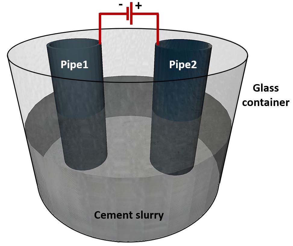
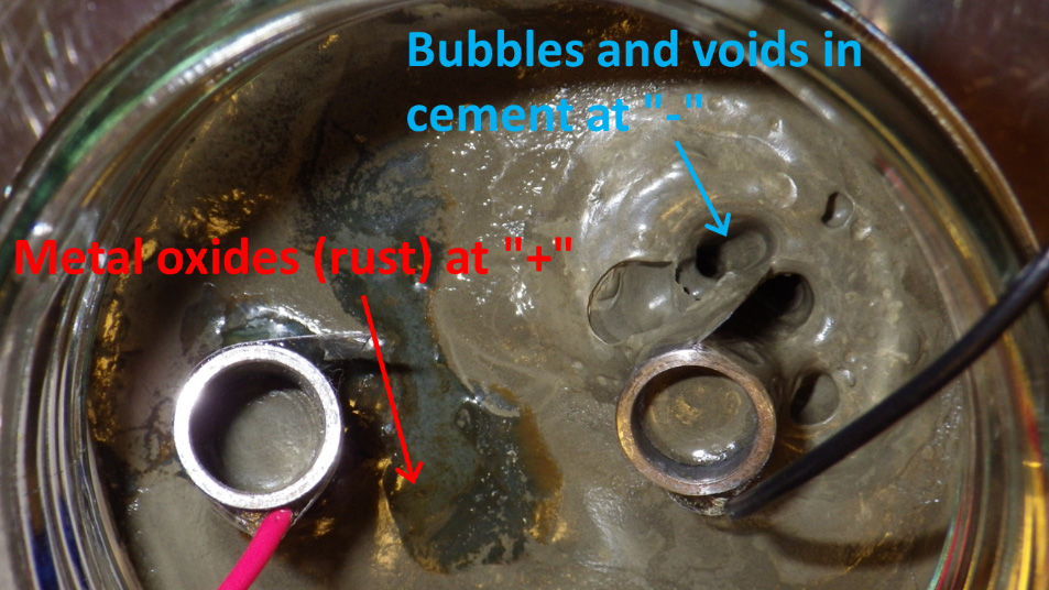
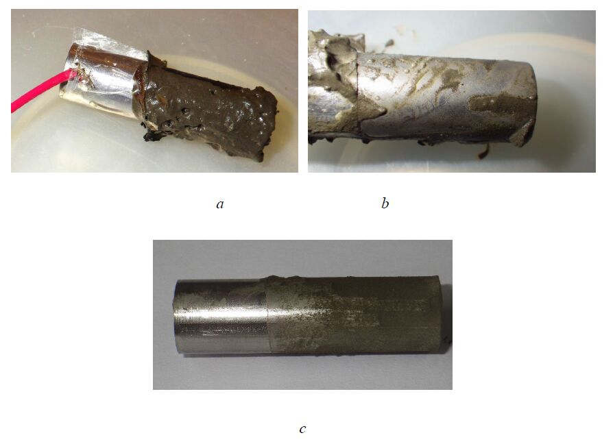
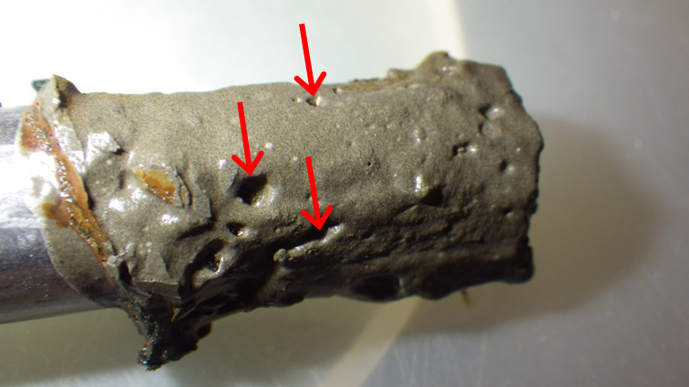
Citation: Alexandre Lavrov, Kamila Gawel, Malin Torsæter. Manipulating cement-steel interface by means of electric field: Experiment and potential applications[J]. AIMS Materials Science, 2016, 3(3): 1199-1207. doi: 10.3934/matersci.2016.3.1199
[1] | Yiwen Tao, Zhenqiang Zhang, Bengbeng Wang, Jingli Ren . Motality prediction of ICU rheumatic heart disease with imbalanced data based on machine learning. Big Data and Information Analytics, 2024, 8(0): 43-64. doi: 10.3934/bdia.2024003 |
[2] | Cai-Tong Yue, Jing Liang, Bo-Fei Lang, Bo-Yang Qu . Two-hidden-layer extreme learning machine based wrist vein recognition system. Big Data and Information Analytics, 2017, 2(1): 59-68. doi: 10.3934/bdia.2017008 |
[3] | Tieliang Gong, Qian Zhao, Deyu Meng, Zongben Xu . Why Curriculum Learning & Self-paced Learning Work in Big/Noisy Data: A Theoretical Perspective. Big Data and Information Analytics, 2016, 1(1): 111-127. doi: 10.3934/bdia.2016.1.111 |
[4] | M Supriya, AJ Deepa . Machine learning approach on healthcare big data: a review. Big Data and Information Analytics, 2020, 5(1): 58-75. doi: 10.3934/bdia.2020005 |
[5] | Maria Gabriella Mosquera, Vlado Keselj . Identifying electronic gaming machine gambling personae through unsupervised session classification. Big Data and Information Analytics, 2017, 2(2): 141-175. doi: 10.3934/bdia.2017015 |
[6] | Bill Huajian Yang . Resolutions to flip-over credit risk and beyond-least squares estimates and maximum likelihood estimates with monotonic constraints. Big Data and Information Analytics, 2018, 3(2): 54-67. doi: 10.3934/bdia.2018007 |
[7] | Bill Huajian Yang, Jenny Yang, Haoji Yang . Modeling portfolio loss by interval distributions. Big Data and Information Analytics, 2020, 5(1): 1-13. doi: 10.3934/bdia.2020001 |
[8] | Ricky Fok, Agnieszka Lasek, Jiye Li, Aijun An . Modeling daily guest count prediction. Big Data and Information Analytics, 2016, 1(4): 299-308. doi: 10.3934/bdia.2016012 |
[9] | Bill Huajian Yang . Modeling path-dependent state transitions by a recurrent neural network. Big Data and Information Analytics, 2022, 7(0): 1-12. doi: 10.3934/bdia.2022001 |
[10] | Marco Tosato, Jianhong Wu . An application of PART to the Football Manager data for players clusters analyses to inform club team formation. Big Data and Information Analytics, 2018, 3(1): 43-54. doi: 10.3934/bdia.2018002 |
Sepsis [1] is defined as a life-threatening clinical syndrome characterized by organ dysfunction due to an imbalanced bodily response to infection. Each year in the United States (US), severe sepsis and septic shock [2] affects 750,000 patients, with a mortality rate of up to 30%. Over half of these patients are admitted to the intensive care unit (ICU), accounting for 10% of all ICU deaths and 20% to 30% of all hospital deaths, resulting in annual healthcare costs of $15.4 billion within the US [3,4,5]. Many nations have analyzed and projected the sepsis mortality rates in their respective countries. For instance, Weng et al. [6] conducted a study on sepsis in China, and revealed significant regional disparities in sepsis-related deaths. Their multilevel analysis indicated that the male gender, advancing age, and comorbidities were independently associated with increased sepsis-related mortality. Fleischmann et al. [7] investigated sepsis mortality in Germany, and found that infection and sepsis were significant causes of hospitalization and death. Prest et al. [8] examined sepsis deaths in the US from 2005 to 2018, and observed that mortality is influenced by race and geographic location. Furthermore, even after discharge, sepsis patients are prone to complications and sequelae that can compromise their health and elevate their 90-day mortality risk. Consequently, sepsis can be regarded as a global public health concern. Given the high mortality rate and economic burden associated with sepsis, timely and effective risk assessments and treatments have become particularly crucial.
A timely sepsis treatment necessitates an early risk assessment [9,10,11] of the patient, highlighting the importance of an effective scoring system for clinicians to identify high-risk patients and to estimate the likelihood of death. Various severity scores [12] are widely used in ICUs to assess the disease severity and prognostic outcomes. However, when it comes to diagnosing sepsis, the clinical application of these scores remains limited. This is due to the complex pathogenesis of sepsis and the inadequacy of relying on a single scoring system. For instance, the acute physiology and chronic health evaluation II (APACHE II) score [13] underestimates the risk of death in sepsis patients in the ICU. Similarly, the simplified acute physiological scoring II (SAPS II) [14] has proven ineffective in external validation studies, further emphasizing the need for more accurate and comprehensive assessment tools in sepsis diagnoses.
Given these limitations, the exploration of new predictive models, particularly those based on machine learning, has become imperative. Numerous researchers have developed sepsis mortality prediction models that leverage machine learning algorithms [15,16,17,18]. These models tend to focus on patients with severe sepsis and septic shock, though they exhibit a poor specificity for sepsis patients. William et al. [19] constructed a mortality risk model that utilized laboratory data and clinical indicators, and demonstrated the feasibility of assessing the sepsis patients' death risk. Nevertheless, most of these models employ either traditional machine learning or unsupervised learning algorithms, which often lack interpretability. To address this issue, we have established a sepsis mortality risk scoring card inspired by financial scoring cards. In this scoring card, each feature is assigned a score within a specific range, and the final death risk is determined by summing these scores, providing a more interpretable and comprehensive assessment tool for sepsis diagnosis.
In this paper, drawing inspiration from financial scoring cards, we develop a sepsis mortality risk scoring card that leverages machine learning techniques, specifically a logistic regression, to identify high-risk sepsis patients upon admission to the ICU. By incorporating easily accessible clinical and laboratory data routinely collected within the first 24 hours of ICU admission, our proposed scoring card aims to provide clinicians with a comprehensive and concise tool to promptly assess the sepsis patients' mortality risk and guiding early intervention to ultimately improve the patient outcomes.
Our method to predict the sepsis mortality risk was modeled and tested on the electronic health record (EHR) data from the Medical Information Mart for Intensive Care Ⅲ (MIMIC Ⅲ) database, version 1.4 [20]. We have obtained ethics approval (registration code: 9641799), which granted us access to use this data. From the MIMIC Ⅲ database, we extracted information on patients admitted to the ICU with sepsis, diagnosed according to the Sepsis 3.0 criteria—specifically, those with suspected infection and a sequential organ failure assessment (SOFA) score of 2 or higher. The primary outcome measure was whether these sepsis patients succumbed within 31 days. The label indicated whether the sepsis patients succumbed within 31 days, where "1" denoted patient survival, and "0" signified death.
We excluded patients based on the following criteria:
1) Non-adults (aged 12 years or younger);
2) Patients with multiple hospital admissions;
3) Patients whose infection occurred within 24 hours prior to ICU admission; and
4) Patients whose infection occurred more than 24 hours after ICU admission.
After identifying the study population, we subsequently extracted relevant physiological and laboratory data from the MIMIC Ⅲ database.
In this section, we made use of the structured query language (SQL) to pinpoint sepsis patients who met the diagnostic criteria set forth by sepsis 3.0. Following this identification, we proceeded to collect the physiological and laboratory data from the first 24 hours of their ICU admission. The collected basic information encompassed details such as age, sex, race, and admission_type.
The vital signs collected included the following: heart rate (HR), respiration rate (RR), systolic blood pressure (SBP), diastolic blood pressure (DBP), mean arterial pressure (MAP), body temperature (Tem), and oxygen saturation (Spo2).
The laboratory data collected included the following: white blood cell count (WBC), blood lactic acid (Lactate), potassium, serum creatinine (Creatinine), Platelets, Blood Urea Nitrogen (BUN), Sodium Ions (Sodium), chloride ions (Chloride), glucose, international standardized ratio (INR), hemoglobin, hematocrit, and anion space (Anion).
The traditional severity scores include: Oxford acute illness severity score (OASIS), logistic organ dysfunction system (LODS), sequential organ failure assessment (SOFA), system inflammatory reaction syndrome (SIRS), and quick SOFA (qSOFA).
All variables were recorded during the first 24h of ICU admission.
After collecting the data, necessary preprocessing was required due to potential issues such as missing values, outliers, and correlations among features that existed in the raw data. When extracted data remains unprocessed, it frequently gives rise to several issues. For instance, disparities in dimensions hinder direct comparisons. The presence of extreme values and outliers within the dataset diminishes its usability. The correlation among features often results in redundancies, thereby undermining the model's efficacy. Moreover, missing values in the data necessitate varying approaches for either imputation or deletion. Consequently, feature engineering becomes imperative to enhance data utilization and the model accuracy.
We need to preprocess the data with a weight of evidence (WOE) encoding. It is a recoding method applied to independent variables. To perform WOE coding on the variables, we first need to use chi-square boxes to group the variables. Chi-square binning is a bottom-up (i.e., pooling-based) method of data discretization that relies on a chi-square test: the adjacent bins with the smallest chi-square values are pooled together until a certain stopping condition is met. After grouping, for the i-th group, the calculation formula of the WOE is as follows:
WOEi=ln(pyipni)=ln(#yi/#yT#ni/#nT)=ln(#yi/#ni#yT/#nT) | (1) |
Among them, pyi represents the proportion of surviving patients in a particular group relative to all surviving patients in the entire sample (analogous to surviving patients in a medical context). Similarly, pni signifies the proportion of deceased patients in that group compared to all deceased patients in the sample. The variables #yi, #ni, #yT, and #nT denote the number of surviving patients in the group, the number of deceased patients in the group, the total number of surviving patients in the entire sample, and the total number of deceased patients in the entire sample, respectively. The WOE embodies the ratio of surviving to deceased patients in the present group, juxtaposed with this ratio across the entire sample. A higher WOE value indicates a more significant disparity, suggesting that the specific group exerts a greater influence on the dependent variables.
In the binary classification problem of machine learning, the information value (Ⅳ) primarily serves to encode the input variables and to assess their predictive capability. The Ⅳ of a characteristic variable signifies its ability to predict, and its computation relies on the WOE:
IVi=(pyi−pni)×WOEi | (2) |
The Ⅳ value of the variable is obtained by adding the Ⅳs of each group, IV=∑IVi. The calculation of the Ⅳ value is the WOE multiplication coefficient, and this coefficient takes the proportion of the samples in this group to the overall sample into account. The lower the proportion, the lower the contribution of this group is to the overall predictive ability of the variable. Therefore, a reasonable indicator to judge the predictive ability can be obtained. By applying WOE encoding and the Ⅳ value calculation, we can effectively address the extreme values and redundant features within the data, thereby laying a solid foundation for the subsequent model development.
In this paper, we used the Python programming language (version 3.7.0) for data processing. The main packages used are numpy (version 1.19.2) and pandas (version 1.1.5).
Our proposed predictive model uses the individual patient data available within 24 hours of one admission to the ICU and generates the probability of death within 31 days. This prediction task can be solved by various statistical and machine learning models. In the current study, we evaluated a logistic regression, XGBoost, K-Nearest neighbor (KNN), decision tree, and support vector machines on the laboratory datasets. XGBoost is the latest implementation of a gradient tree enhancement system, which includes combining many "weak" decision tree predictors into a single powerful predictor. In view of the strong interpretability of the logistic regression algorithm, we used it to construct the sepsis death risk score card. In addition, to prevent over-fitting, we used a hierarchical five-fold-cross validation to evaluate the generalize ability of our prediction model. The main evaluation indexes of the model were accuracy, area under the curve (AUC), specificity, and sensitivity. Machine learning training and evaluation were performed in Python, using the sklearn (version 0.24.1) and scorecardpy (version 1.1.9.2) packages. The analysis code for this study is available on reasonable request.
The sample with multiple missing values was deleted, and the variables with missing data less than 5% were filled with an average interpolation. Then, Pearson's correlation was calculated for the continuous variables. A correlation analysis found that the correlation between hemoglobin and hematocrit (0.96), chloride and sodium (0.70), and the BUN and creatinine (0.68) variables were high. The two variables with high correlations were deleted according to the Ⅳ value (the one with the higher Ⅳ value is retained). Figure 1 illustrates the correlation among various features, providing a visual representation of the interrelationships between different characteristics within the dataset: the darker the color, the higher the correlation. The Ⅳ value can be used to describe the predictive ability of the variables, and the relationship between the Ⅳ value and the predictive ability is as follows: Ⅳ value <= 0.02, no predictive ability; 0.02 <= Ⅳ value <= 0.1, weak predictive ability; 0.1 <= Ⅳ value <= 0.3, moderate predictive ability; 0.3 <= Ⅳ value <= 0.5, strong predictive ability; and 0.5 <= Ⅳ value <= 1, doubtful. Finally, we selected 9 variables with an Ⅳ value greater than 0.1 as the input variables.
The variables that ultimately entered the model and demonstrated strong predictive capabilities for labels include Anion, INR, RR, BUN, HR, admission_type, lactate, age, and Tem.
A preliminary study conducted on the MIMIC Ⅲ database identified 37,721 hospitalized patients who had only one ICU admission. Among these, 30,075 patients aged 12 years or older were selected for further analysis. However, 5004 patients were excluded due to infections that occurred either too early or too late in their hospital stay, 12,616 patients did not meet the sepsis 3.0 criteria, and another 4536 patients were excluded due to incomplete basic data. This resulted in a final cohort of 7919 patients, among whom 1665 died, yielding a mortality rate of 20%. Table 1 provides an overview of the demographic and clinical characteristics of all patients included in the analysis, grouped by survivors and non-survivors. For the continuous variables, the mean (± standard deviation) is presented, while for the categorical variables, the number and proportion are shown.
Survivors (n = 6254) | Non–survivors (n = 1665) | |
Demographic | ||
Age (yr) | 63.5 (45.8–81.2) | 69.5 (52.4–86.3) |
Admission_type (n, %) | ||
Elective | 1079 (17.3) | 31 (1.9) |
Urgent | 5087 (81.3) | 1604 (96.3) |
Emergency | 88 (1.4) | 30 (1.8) |
Basic Vital Signs | ||
Heart Rate | 103.1 (83.1–123.0) | 111.6 (87.1–135.9) |
Respiratory Rate | 26.0 (19.4–32.8) | 29.2 (22.0–36.3) |
Temperature | 37.5 (36.7–38.4) | 37.2 (36.1–38.5) |
Laboratory Indicators | ||
Lactate | 3.0 (0.8–5.2) | 4.9 (0.9–9.0) |
INR | 1.6 (0.2–3.0) | 2.2 (0.1–4.3) |
Anion | 15.8 (11.1–20.6) | 19.6 (13.2–26.0) |
BUN | 17.7 (5.5–50.2) | 40.7 (12.8–68.9) |
Severity Score | ||
SOFA | 5 (3–8) | 8 (4–12) |
SIRS | 2 (1–4) | 3 (2–4) |
OASIS | 34 (26–42) | 43 (34–52) |
LODS | 5 (3–7) | 8 (5–11) |
qSOFA | 2 (1–8) | 2 (1–5) |
The distribution of our variables is significantly skewed. Introducing these variables into the model without any preprocessing would result in information dispersion, thereby hindering an accurate prediction of the mortality risk. To visualize this skewness, we have crafted several variable box plots, which are exhibited in Figure 2. Evidently, these variables possess numerous extreme values. Based on their predictive capacity for the mortality rate, each feature has been segmented into 2–4 categories or "boxes".
The Ⅳ value of the final retained variables stands as follows: HR: 0.138, Tem: 0.139, age: 0.138, RR: 0.233, INR: 0.254, admission_type: 0.370, BUN: 0.380, anion: 0.476, and lactate: 0.380. For Ⅳ values of other variables, refer to Table 2. These explanatory variables demonstrate a remarkable predictive strength, and their Ⅳ values reflect the significance of these features.
variables | Ⅳ value |
Potassium | 0.0114 |
DBP | 0.0124 |
Sex | 0.0146 |
SBP | 0.0217 |
MAB | 0.0224 |
Platelet | 0.028 |
Gcs | 0.0323 |
Sodium | 0.0451 |
Spo2 | 0.0499 |
WBC | 0.0499 |
Chloride | 0.0559 |
Glucose | 0.0662 |
Hematocrit | 0.0681 |
Hemoglobin | 0.0799 |
Age | 0.1375 |
HR | 0.1375 |
Tem | 0.1387 |
RR | 0.2328 |
INR | 0.2538 |
Creatinine | 0.2944 |
Admission_Type | 0.3689 |
Bun | 0.3794 |
Lactate | 0.3804 |
Anion | 0.4756 |
The boxing of variables is illustrated in Figure 3. For instance, in part (c), the variable BUN is partitioned into four ranges: less than 18, 18–24, 24–34, and greater than 34. Within the figure, red signifies deceased patients, while blue represents the survivors. On the bar chart, the notation (32.4%, 2564) indicates that 2564 patients had a blood urea nitrogen index value less than 18, constituting 32.4% of the total population. The 89.4% on the line chart signifies that among these patients, 89.4% survived. Likewise, 83.7% implies that out of the 1689 patients (comprising 21.4% of the total sample) with a BUN value in the range of [18,24], the survival rate was 83.7%.
To address the issue of the imbalanced proportions of positive and negative samples in datasets, the synthetic minority over-sampling technique (SMOTE) upsampling was employed. The dataset was randomly partitioned into two subsets at a 3 : 7 ratio, where the larger subset was designated for model training and evaluation, and the smaller one was reserved for the final model validation. All nine variables were incorporated into the model, and the evaluation metrics included the AUC, sensitivity, specificity, and accuracy. Cross-validation revealed that among all tested models, XGBoost exhibited the best performance, achieving an AUC of 0.91. Other models demonstrated a similar respectable performance, with AUCs of 0.81 for the logistic regression, 0.82 for the KNN, 0.82 for the decision tree, and 0.81 for the support vector machine. Figure 4 illustrates the receiver operating characteristic (ROC) curves of each model on the test set, highlighting that XGBoost remained the top performer in the test set, attaining an AUC of 0.91, whereas the AUCs of the other models ranged from 0.8 to 0.85.
We have presented the accuracy, sensitivity, specificity, and AUC of each model on both the training and test sets in Table 3. The ROC curves of each machine learning model are presented in Figure 4. The accuracy provides a straightforward assessment of the model's ability to correctly predict the outcome for the patients. Among the commonly used evaluation indicators, the specificity and sensitivity hold particular significances. The sensitivity reflects the model's ability to identify patients who have passed away, while the specificity demonstrates its capacity to recognize those who have survived. Given the focus of our model on identifying patients at higher risk of mortality, the sensitivity became a crucial metric. Notably, XGBoost and the decision tree exhibited stronger sensitivities, with values of 0.84 and 0.78, respectively.
Accuracy | Sensitivity | Specificity | AUC | ||
Logistic | train | 0.71 | 0.73 | 0.71 | 0.80 |
test | 0.72 | 0.72 | 0.73 | 0.81 | |
XGBoost | train | 0.85 | 0.86 | 0.84 | 0.93 |
test | 0.83 | 0.84 | 0.82 | 0.91 | |
K-Neighbors | train | 0.78 | 0.81 | 0.75 | 0.87 |
test | 0.74 | 0.74 | 0.73 | 0.82 | |
Decision Tree | train | 0.74 | 0.79 | 0.69 | 0.82 |
test | 0.73 | 0.78 | 0.69 | 0.82 | |
Support Vector | train | 0.74 | 0.74 | 0.74 | 0.82 |
test | 0.74 | 0.72 | 0.75 | 0.81 |
Currently, numerous scholars have developed models to predict the mortality risk among sepsis patients. In this section, we compare our model with several previously published models to demonstrate its efficacy. Table 4 summarizes the comparison outcomes.
Model | Variables number | Sample size | ML model | AUC |
Model1 | 9 | 7919 | XGBoost | 0.91 |
Model2 | 5 | 159 | Logistic | 0.82 |
Model3 | 13 | 11101 | LASSO | 0.78 |
Model4 | 20 | 1344 | XGBoost | 0.84 |
Model5 | 20 | 9954 | Random forest | 0.86 |
Model 1: Wan et al. [21] employed five medical examination indicators, including PCT and interleukin 6, and used a logistic regression to achieve an AUC of 0.82. However, their model relies on indicators that are only detectable when the disease progresses to a severe stage, thus limiting early prediction.
Model 2: Zhang et al. [22] used MIMIC Ⅲ data to construct a Lasso model, and achieved an AUC of 0.78. Their approach of dividing variables into only two categories resulted in some information loss.
Model 3: William's team [23] created an XGBoost model using comprehensive patient data and emergency room visits, and achieved an AUC of 0.84 on the validation set.
Model 4: Taylor et al. [24] built a model that included the random forest, logistic regression, and the classification and regression tree (CART) models, utilizing patient data from four EDs. The random forest model performed the best, and yielded an AUC of 0.86.
In contrast, our model outperforms these existing models due to our unique feature processing technique. By employing chi-square classification for the feature selection, we maximized the data utilization and facilitated the construction of a scoring card, thereby enhancing the predictive accuracy. Our XGBoost model achieved an AUC of 0.91, demonstrating its superiority.
Based on the fundamental principles of a logistic regression, let us denote the probability of survival as p, and consequently, the probability of mortality as 1-p. According to the financial scorecard methodology, odds represents the ratio between the number of creditworthy (good) customers and uncreditworthy (bad) customers, where the creditworthy customers are assigned higher scores. When adapting this framework to assess the mortality risk scores in a medical context, we consider that the severity of a disease directly correlates with an increased mortality rate. Therefore, patients with more severe conditions, which indicate a higher mortality risk, should receive higher scores as an early warning indicator. In this analogy, a "good customer" corresponds to a patient whose final outcome is unfortunately death, while a "bad customer" represents a patient who survives. With this paradigm, we can derive the following:
odds=p1−p. | (3) |
The probability of survival can be expressed as follows:
p=odds1+odds. | (4) |
Our score can be expressed as a linear expression of the logarithm of the ratio, and the score card scale can be set accordingly:
Score=A−Bln(odds). | (5) |
As we can see from the formula, the higher the probability of death, the higher the score. We need the following two assumptions to solve for A and B:
(1) Set the expected score to be S0 when the odd is θ0; and
(2) When the θ0 is doubled, the change in the score is PDO. By substituting the hypothesis into Eq (3), we can obtain the following:
{S0=A−Bln(θ0)S0+PDO=A−Bln(2θ0). | (6) |
The values A and B are obtained by solving the following formula:
{A=S0+Bln(θ0)B=PDOln2. | (7) |
Additionally, the logistic regression model is expressed as follows:
ln(odds)=b+ω1⋅x1+ω2⋅x2+⋯+ωn⋅xn. | (8) |
The formula for the score can be rewritten as follows:
Score=A−B(b+ω1⋅x1+ω2⋅x2+⋯+ωn⋅xn). | (9) |
We set the parameters as S0 = 10 and PDO = 2. The final scoring card, which is presented in
Table 5, facilitates the assessment of each patient's score, with higher scores indicating an elevated risk of mortality. In terms of the admission type, elective hospitalizations are associated with a lower mortality risk, hence the assigned score of –3, whereas emergency hospitalizations, due to their higher mortality risk, received a score of 2. Given that the mortality rate in the dataset is 20%, the corresponding odds are calculated to be 4. This allows us to determine the score values associated with different probabilities of death. Specifically, a score of 12 corresponds to a 33% risk of death, 14 points indicate a 50% risk, and 17 points signify a 75% risk of death. We categorize the scores into four risk levels: low risk ([2, 12)), medium-low risk ([12, 14)), medium-high risk ([14, 17)), and high risk ([17, 26)), with the latter representing the highest risk of death.
Characteristics | Numerical range | Score |
RR (b/min) | < 20 | 0 |
20–30 | 1 | |
> 30 | 3 | |
BUN (mg/dL) | < 18 | 0 |
18–24 | 1 | |
24–34 | 2 | |
> 34 | 3 | |
INR | < 2 | 1 |
> 2 | 3 | |
Age | < 46 | 0 |
46–76 | 1 | |
76–86 | 3 | |
> 86 | 4 | |
Anion (mEq/L) | < 19 | 1 |
19–24 | 2 | |
> 24 | 3 | |
Admission_type | ELECTⅣE | –3 |
EMERGENCY, URGENT |
2 | |
Tem (C) | < 36 | 4 |
36–37 | 2 | |
> 37 | 1 | |
HR (b/min) | < 115 | 1 |
> 115 | 2 | |
Lactate (mmol/L) | < 4 | 1 |
4–6 | 2 | |
6–9 | 3 | |
> 9 | 5 |
Using this scoring system, we analyzed 7919 sepsis patients from the dataset, as illustrated in Figure. Our findings reveal a clear trend: patients who eventually succumbed to the illness tended to have significantly higher scores, with only 12.2% falling into the low-risk category. Conversely, patients who survived had predominantly lower scores, with just 7.8% classified as high-risk. The numbers presented in the table further demonstrate the effectiveness of this scoring system to distinguish between patients based on their risk levels. For instance, 3128 represents the number of surviving patients with low-risk scores, accounting for 50% of all survivors, whereas 203 denotes the number of deceased patients with low-risk scores, constituting 12.2% of all fatalities. These results closely align with the actual outcomes, underscoring the model's effectiveness.
To further validate the robustness of our model, we not only benchmarked it against other predictive models, but also conducted a comparative analysis with existing medical scoring systems. Our findings reveal that our model outperforms the currently available scoring systems. For illustrative purposes, the AUC curve of our scorecard model is exhibited in Figure 6. As evident from Figure 7, the existing medical scores exhibit varying degrees of sensitivity and specificity. Among them, LODS stands out with an AUC of 0.78, along with a high sensitivity of 0.86. However, its specificity is relatively low at 0.48. Notably, the AUC of our scorecard model, 0.79, surpasses the highest LODS score, 0.78, among the other medical assessments. Derived from a logistic regression, LODS proves to be a useful tool, but it falls short of being the ultimate predictor of mortality risk in the sepsis patients. The OASIS model demonstrates a more balanced approach with an AUC of 0.75, a sensitivity of 0.76, and a specificity of 0.64. While its performance surpasses other medical scores, it slightly lags behind the logistic regression models. It's worth noting that the specificity of the SOFA scoring model might be skewed due to its limitation in patient screening (SOFA >= 2). On the other hand, the QSOFA score, primarily designed for use outside the ICU, may not provide accurate predictions for patients within the ICU setting. Both the OASIS and LODS scores assess the disease severity, though neither is tailored specifically to sepsis. Given these limitations and the unique challenges posed by sepsis, the development of this mortality risk scoring system specifically designed for sepsis patients in this paper holds a strong practical significance.
Our study showcased the utilization of machine learning models to predict 31-day mortality among sepsis patients admitted to the ICU, with several significant findings and implications.
1) Precision of Machine Learning Models: We established the precision of machine learning-driven models in forecasting 31-day mortality among sepsis patients. Our study demonstrated that the XGBoost model performed exceptionally well, with an AUC of 0.91, and outperformed other traditional machine learning algorithms and clinical risk scores.
2) Development of Mortality Risk Scoring System: By harnessing various methodologies, including a logistic regression, we formulated a mortality risk scoring system specifically tailored for sepsis patients. This scoring system integrated only nine straightforward variables routinely documented in clinical environments, and eliminated the need for manual data input [19].
3) Comparison with Existing Clinical Risk Scores: Our scoring system outperformed several widely-used clinical risk scores, such as qSOFA, LODS, OASIS, SIRS, and SOFA [25,26,27,28,29].
4) Applicability and Limitations: Although our model demonstrated a commendable performance, several limitations exist. First, as with any retrospective analysis, the included data and its precision hinge on the original ICU records, making it prone to potential biases. Second, our focus was on sepsis patients admitted to the ICU, thus limiting the generalizability of our findings to other patient populations. Lastly, the conversion of continuous variables into discrete ones through variable binning might have slightly compromised the prediction accuracy.
Future Directions: Prospective studies are needed to assess the efficacy of our approach and its potential to enhance the clinical outcomes in patients at a high risk of sepsis. Furthermore, external validations of our model in different patient populations are needed to confirm its generalizability.
This study retrospectively analyzed the MIMIC Ⅲ database, and utilized sepsis 3.0 diagnostic criteria alongside the first-day laboratory indicators and clinical data of patients. Through a machine learning technology, we constructed a mortality risk scoring card specifically tailored for sepsis patients. This scoring system outperformed several existing medical scores. By leveraging easily accessible indicators, this paper enabled the rapid determination of death risk scores shortly after patients are admitted to the ICU. This timely assessment aids physicians in quickly understanding a patient's physical condition, potentially leading to an improved prognosis.
The authors declare they have not used Artificial Intelligence (AI) tools in the creation of this article.
This work was supported by the National Natural Science Foundation of China under the Grant Nos. 11702250 and the Key Scientific Research Projects of Colleges and Universities in Henan Province under Grant No.22A520010.
The authors declare that they have no conflict of interest with respect to the research, authorship, and publication of the article.
[1] | Nelson EB, Guillot D (2006) Well cementing: Schlumberger. |
[2] |
Kjøller C, Torsæter M, Lavrov A, et al. (2016) Novel experimental/numerical approach to evaluate the permeability of cement-caprock systems. Int J Greenhouse Gas Control 45: 86–93. doi: 10.1016/j.ijggc.2015.12.017
![]() |
[3] | Lavrov A, Cerasi P (2013) Numerical modeling of tensile thermal stresses in rock around a cased well caused by injection of a cold fluid. ARMA paper 13-306 presented at the 47th US Rock Mechanics/Geomechanics Symposium held in San Francisco, CA, USA. |
[4] | Drever JI (1969) The separation of clay minerals by continuous particle electrophoresis. Am Mineral 54: 937–942. |
[5] | Hoxha BB, Sullivan G, van Oort E, et al. (2016) Determining the zeta potential of intact shales via electrophoresis. SPE paper 180097 presented at the SPE Europec featured at the 78th EAGE Conference and Exhibition held in Vienne, Austria. |
[6] |
Nachbaur L, Mutin JC, Nonat A, et al. (2001) Dynamic mode rheology of cement and tricalcium silicate pastes from mixing to setting. Cement Concrete Res 31: 183–192. doi: 10.1016/S0008-8846(00)00464-6
![]() |
[7] |
Roy S, Cooper GA (1993) Prevention of bit balling in shales - preliminary results. SPE Drill Completion 8: 195–200. doi: 10.2118/23870-PA
![]() |
[8] | Bourgoyne Jr. AT, Millheim KK, Chenevert ME, et al. (1991) Applied Drilling Engineering. Richardson: Society of Petroleum Engineers 502. |
[9] |
Lavrov A, Todorovic J, Torsæter M (2016) Impact of voids on mechanical stability of well cement. Energy Procedia 86: 401–410. doi: 10.1016/j.egypro.2016.01.041
![]() |
[10] | Todorovic J, Gawel K, Lavrov A, et al. (2016) Integrity of downscaled well models subject to cooling. SPE paper 180025 presented at the SPE Bergen One Day Seminar held in Bergen, Norway. |
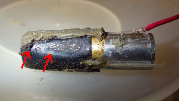
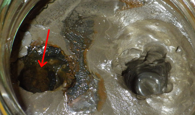
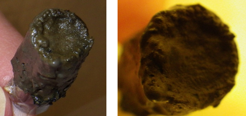
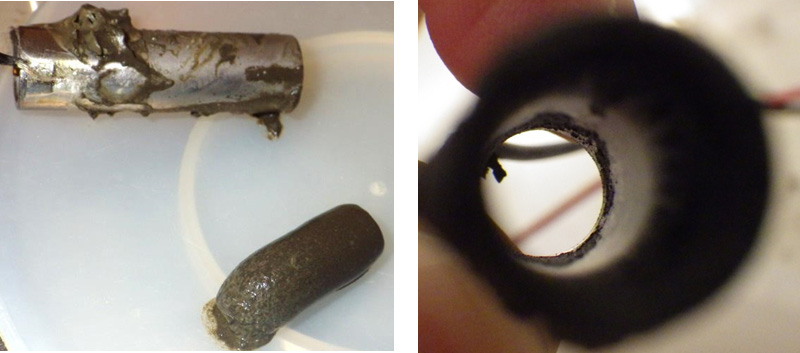
Survivors (n = 6254) | Non–survivors (n = 1665) | |
Demographic | ||
Age (yr) | 63.5 (45.8–81.2) | 69.5 (52.4–86.3) |
Admission_type (n, %) | ||
Elective | 1079 (17.3) | 31 (1.9) |
Urgent | 5087 (81.3) | 1604 (96.3) |
Emergency | 88 (1.4) | 30 (1.8) |
Basic Vital Signs | ||
Heart Rate | 103.1 (83.1–123.0) | 111.6 (87.1–135.9) |
Respiratory Rate | 26.0 (19.4–32.8) | 29.2 (22.0–36.3) |
Temperature | 37.5 (36.7–38.4) | 37.2 (36.1–38.5) |
Laboratory Indicators | ||
Lactate | 3.0 (0.8–5.2) | 4.9 (0.9–9.0) |
INR | 1.6 (0.2–3.0) | 2.2 (0.1–4.3) |
Anion | 15.8 (11.1–20.6) | 19.6 (13.2–26.0) |
BUN | 17.7 (5.5–50.2) | 40.7 (12.8–68.9) |
Severity Score | ||
SOFA | 5 (3–8) | 8 (4–12) |
SIRS | 2 (1–4) | 3 (2–4) |
OASIS | 34 (26–42) | 43 (34–52) |
LODS | 5 (3–7) | 8 (5–11) |
qSOFA | 2 (1–8) | 2 (1–5) |
variables | Ⅳ value |
Potassium | 0.0114 |
DBP | 0.0124 |
Sex | 0.0146 |
SBP | 0.0217 |
MAB | 0.0224 |
Platelet | 0.028 |
Gcs | 0.0323 |
Sodium | 0.0451 |
Spo2 | 0.0499 |
WBC | 0.0499 |
Chloride | 0.0559 |
Glucose | 0.0662 |
Hematocrit | 0.0681 |
Hemoglobin | 0.0799 |
Age | 0.1375 |
HR | 0.1375 |
Tem | 0.1387 |
RR | 0.2328 |
INR | 0.2538 |
Creatinine | 0.2944 |
Admission_Type | 0.3689 |
Bun | 0.3794 |
Lactate | 0.3804 |
Anion | 0.4756 |
Accuracy | Sensitivity | Specificity | AUC | ||
Logistic | train | 0.71 | 0.73 | 0.71 | 0.80 |
test | 0.72 | 0.72 | 0.73 | 0.81 | |
XGBoost | train | 0.85 | 0.86 | 0.84 | 0.93 |
test | 0.83 | 0.84 | 0.82 | 0.91 | |
K-Neighbors | train | 0.78 | 0.81 | 0.75 | 0.87 |
test | 0.74 | 0.74 | 0.73 | 0.82 | |
Decision Tree | train | 0.74 | 0.79 | 0.69 | 0.82 |
test | 0.73 | 0.78 | 0.69 | 0.82 | |
Support Vector | train | 0.74 | 0.74 | 0.74 | 0.82 |
test | 0.74 | 0.72 | 0.75 | 0.81 |
Model | Variables number | Sample size | ML model | AUC |
Model1 | 9 | 7919 | XGBoost | 0.91 |
Model2 | 5 | 159 | Logistic | 0.82 |
Model3 | 13 | 11101 | LASSO | 0.78 |
Model4 | 20 | 1344 | XGBoost | 0.84 |
Model5 | 20 | 9954 | Random forest | 0.86 |
Characteristics | Numerical range | Score |
RR (b/min) | < 20 | 0 |
20–30 | 1 | |
> 30 | 3 | |
BUN (mg/dL) | < 18 | 0 |
18–24 | 1 | |
24–34 | 2 | |
> 34 | 3 | |
INR | < 2 | 1 |
> 2 | 3 | |
Age | < 46 | 0 |
46–76 | 1 | |
76–86 | 3 | |
> 86 | 4 | |
Anion (mEq/L) | < 19 | 1 |
19–24 | 2 | |
> 24 | 3 | |
Admission_type | ELECTⅣE | –3 |
EMERGENCY, URGENT |
2 | |
Tem (C) | < 36 | 4 |
36–37 | 2 | |
> 37 | 1 | |
HR (b/min) | < 115 | 1 |
> 115 | 2 | |
Lactate (mmol/L) | < 4 | 1 |
4–6 | 2 | |
6–9 | 3 | |
> 9 | 5 |