Figure 1.
Schematic diagram of the LMFS: (a) nodal distribution and (b) local subdomain.
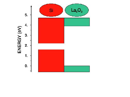
Citation: Alberto Debernardi. Ab initio calculation of band alignment of epitaxial La2O3 on Si(111) substrate[J]. AIMS Materials Science, 2015, 2(3): 279-293. doi: 10.3934/matersci.2015.3.279
| [1] | K. Wayne Forsythe, Cameron Hare, Amy J. Buckland, Richard R. Shaker, Joseph M. Aversa, Stephen J. Swales, Michael W. MacDonald . Assessing fine particulate matter concentrations and trends in southern Ontario, Canada, 2003–2012. AIMS Environmental Science, 2018, 5(1): 35-46. doi: 10.3934/environsci.2018.1.35 |
| [2] | Suprava Ranjan Laha, Binod Kumar Pattanayak, Saumendra Pattnaik . Advancement of Environmental Monitoring System Using IoT and Sensor: A Comprehensive Analysis. AIMS Environmental Science, 2022, 9(6): 771-800. doi: 10.3934/environsci.2022044 |
| [3] | Muhammad Rendana, Wan Mohd Razi Idris, Sahibin Abdul Rahim . Clustering analysis of PM2.5 concentrations in the South Sumatra Province, Indonesia, using the Merra-2 Satellite Application and Hierarchical Cluster Method. AIMS Environmental Science, 2022, 9(6): 754-770. doi: 10.3934/environsci.2022043 |
| [4] | Shagufta Henna, Mohammad Amjath, Asif Yar . Time-generative AI-enabled temporal fusion transformer model for efficient air pollution sensor calibration in IIoT edge environments. AIMS Environmental Science, 2025, 12(3): 526-556. doi: 10.3934/environsci.2025024 |
| [5] | Suwimon Kanchanasuta, Sirapong Sooktawee, Natthaya Bunplod, Aduldech Patpai, Nirun Piemyai, Ratchatawan Ketwang . Analysis of short-term air quality monitoring data in a coastal area. AIMS Environmental Science, 2021, 8(6): 517-531. doi: 10.3934/environsci.2021033 |
| [6] | Carolyn Payus, Siti Irbah Anuar, Fuei Pien Chee, Muhammad Izzuddin Rumaling, Agoes Soegianto . 2019 Southeast Asia Transboundary Haze and its Influence on Particulate Matter Variations: A Case Study in Kota Kinabalu, Sabah. AIMS Environmental Science, 2023, 10(4): 547-558. doi: 10.3934/environsci.2023031 |
| [7] | Winai Meesang, Erawan Baothong, Aphichat Srichat, Sawai Mattapha, Wiwat Kaensa, Pathomsorn Juthakanok, Wipaporn Kitisriworaphan, Kanda Saosoong . Effectiveness of the genus Riccia (Marchantiophyta: Ricciaceae) as a biofilter for particulate matter adsorption from air pollution. AIMS Environmental Science, 2023, 10(1): 157-177. doi: 10.3934/environsci.2023009 |
| [8] | Joanna Faber, Krzysztof Brodzik . Air quality inside passenger cars. AIMS Environmental Science, 2017, 4(1): 112-133. doi: 10.3934/environsci.2017.1.112 |
| [9] | Pratik Vinayak Jadhav, Sairam V. A, Siddharth Sonkavade, Shivali Amit Wagle, Preksha Pareek, Ketan Kotecha, Tanupriya Choudhury . A multi-task model for failure identification and GPS assessment in metro trains. AIMS Environmental Science, 2024, 11(6): 960-986. doi: 10.3934/environsci.2024048 |
| [10] | Anna Mainka, Barbara Kozielska . Assessment of the BTEX concentrations and health risk in urban nursery schools in Gliwice, Poland. AIMS Environmental Science, 2016, 3(4): 858-870. doi: 10.3934/environsci.2016.4.858 |
The method of fundamental solutions (MFS) [1,2] is a simple, accurate and efficient boundary-type meshfree approach for the solution of partial differential equations, which uses the fundamental solution of a differential operator as a basis function. Chen et al. [3,4] demonstrated the equivalence between the MFS and the Trefftz collocation method [5] under certain conditions. During the last decades, the MFS has been widely applied to various fields in applied mathematics and mechanics, such as scattering and radiation problems [6], inverse problems [7], non-linear problems [8], and fractal derivative models [9,10]. For more details and applications, the readers are referred to Refs. [11,12,13] and the references therein. In the MFS, the approximation solution is assumed as a linear combination of fundamental solutions. In order to avoid the source singularity of the fundamental solution, this method requires a fictitious boundary outside the computational domain, and places the source points on it. The distance between the fictitious boundary and the real boundary has a certain influence on the calculation accuracy [14,15,16]. To address this issue, many scholars proposed improved methods, such as the singular boundary method [17,18], modified method of fundamental solutions [19], the non-singular method of fundamental solutions [20]. Due to the characteristic of dense matrix, the traditional and improved MFS with "global" discretization is difficult to apply in the large-scale problems with complicated geometries.
Recently, Fan and Chen et al. [21] proposed an improved version of traditional MFS, known as the localized method of fundamental solutions (LMFS), for solving Laplace and biharmonic equations. The LMFS is essentially a localized semi-analytical meshless collocation scheme, and overcomes the limitation of traditional method in applications of complex geometry and large-scale problems. Gu and Liu et al. [22,23,24,25] extended to the LMFS to elasticity, heat conduction and inhomogeneous elliptic problems. Qu et al. [26,27,28] applied the method to the interior acoustic and bending analysis. Wang et al. [29,30,31,32] developed the localized space-time method of fundamental solutions, and resolved the inverse problems. Li et al. [33] used this method to simulate 2D harmonic elastic wave problems. Liu et al. [34] combined the LMFS and the Crank-Nicolson time-stepping technology to address the transient convection-diffusion-reaction equations. Li, Qu and Wang et al. [35,36,37] given the error analysis of the LMFS, and proposed a augmented moving least squares approximation. Like the element-free Galerkin method [38,39] being successfully applied to a large number of partial differential equations, the proposed LMFS belongs to the domain-type meshless method. Unlike the former, the latter is a semi-analytical meshless collocation method with strong form, in which the fundamental solutions are unavoidable. In the LMFS, the whole computational domain is firstly divided into a set of overlapping local subdomains whose boundary could be a circle (for 2D problems) and/or a sphere (for 3D problems). In each of the local subdomain, the classical MFS formulation and the moving least square (MLS) method are applied to the local approximation of variables. This method remains the high accuracy of the traditional MFS, and simultaneously produces a sparse system of linear algebraic equations. Inspired by the LMFS, recently, some new local meshless methods [40,41,42,43,44] have also been proposed.
No methodology is perfect, although the LMFS has achieved varying degrees of success in various fields, it still faces some thorny problems to be solved. As a local semi-analytical meshless technique, the LMFS needs to configure nodes in the whole computational domain and to select the supporting nodes in each local subdomain, which likes the generalized finite difference method [45,46,47]. The node spacing (related to the total number of nodes), the number of supporting nodes and the relationship between them have the certain influence on the accuracy. Fu et al. [48] discussed the selection algorithm of supporting nodes in the generalized finite difference method. However, there are few reports in the literature coordinating the node spacing and the number of supporting nodes in the LMFS.
In this paper, we propose an effective empirical formula to determine the node spacing and the number of supporting nodes in the LMFS for solving 2D potential problems with Dirichlet boundary condition. A reasonable number of supporting nodes can be directly given according to the size of node spacing. The proposed methodology is applicable to both regular and irregular distribution of nodes in arbitrary domain. This study consummates the LMFS and lays a foundation for simulating various engineering problems accurately and stably.
The rest of paper is organized as follows. In Section 2, we give the governing equation and boundary condition of 2D potential problems, and provide the numerical implementation of LMFS. Section 3 introduces the empirical formula of the node spacing and the number of supporting nodes in the LMFS. Section 4 investigates two numerical examples with irregular domain and nodes to illustrate the accuracy and reliability of the empirical formula. Section 5 summarizes some conclusions.
Considering the following 2D potential problem with the Dirichlet boundary condition:
| $ {\nabla ^2}u(x, y) = 0, {\rm{ \;\;\; }}(x, y) \in \Omega , $ | (1) |
| $ u = \bar u(x, y), {\rm{ \;\;\; }}(x, y) \in \Gamma , $ | (2) |
where ${\nabla ^2}$ is the 2D Laplacian, $u(x, y)$ the unknown variable, $\Omega $ the computational domain, $\Gamma = \partial \Omega $ the boundary of domain, and $\bar u(x, y)$ the given function.
According to the ideas of the LMFS, $N = ni + nb$ nodes ${{\boldsymbol{x}}^i}$ $(i = 1, 2, ..., N)$ should be distributed inside the considered domain $\Omega $ and along its boundary $\Gamma $, where ni is the number of interior nodes, nb is the number of boundary nodes. Consider an arbitrary node ${{\boldsymbol{x}}^{(0)}}$ (called the central node), we can find m supporting nodes ${{\boldsymbol{x}}^{(i)}}$ ($i = 1, 2, ..., m$) around the central node ${{\boldsymbol{x}}^{(0)}}$ (see Figure 1 (a)). At the same time, the local subdomain ${\Omega _s}$ can also be defined. Subsequently, the MFS formulation is implemented for the local subdomain. For this purpose, an artificial boundary ${\overset{\lower0.5em\hbox{$\smash{\scriptscriptstyle\frown}$}}{\Omega } _s}$ is selected at a certain distance from the boundary of local subdomain, as shown in Figure 1 (b). On the artificial boundary, $M$ uniformly distributed source points are specified.
For each node in the local subdomain ${\Omega _s}$, the following MFS formulation of numerical solution should be hold
| $ u({\mathit{\boldsymbol{x}}^{(i)}}) = \sum\limits_{j = 1}^M {{\alpha _j}} G({\mathit{\boldsymbol{x}}^{(i)}}, {\mathit{\boldsymbol{s}}^{(j)}}), {\mathit{\boldsymbol{x}}^{(i)}} \in {\Omega _s}, i = 0, 1, ..., m, $ | (3) |
or for brevity
| $ {\mathit{\boldsymbol{u}}^{(i)}} = \sum\limits_{j = 1}^M {{\alpha _j}} {G_{ij}} = {\mathit{\boldsymbol{G}}^{(i)}}\mathit{\boldsymbol{\alpha }}, {\mathit{\boldsymbol{x}}^{(i)}} \in {\Omega _s}, i = 0, 1, ..., m, $ | (4) |
where $\left(\boldsymbol{x}^{(i)}\right)_{i = 0}^{m}$ are the m+1 nodes in the subdomains ${\Omega _s}$, $\left({{\mathit{\boldsymbol{s}}^{(j)}}} \right)_{j = 1}^M$ denote M fictitious source points, $\boldsymbol{\alpha} = \left(\alpha_{1}, \alpha_{2}, \ldots, \alpha_{M}\right)^{T}$ represent the unknown coefficient vector, $G_{i j} = G\left(\boldsymbol{x}^{(i)}, \boldsymbol{s}^{(j)}\right)$ are the fundamental solutions expressed as
| $ G({\mathit{\boldsymbol{x}}^{(i)}}, {\mathit{\boldsymbol{s}}^{(j)}}) = - \frac{1}{{2\pi }}\ln {\left\| {{\mathit{\boldsymbol{x}}^{(i)}}, {\mathit{\boldsymbol{s}}^{(j)}}} \right\|_2}. $ | (5) |
It should be pointed out that the artificial boundary is a circle centered at ${{\boldsymbol{x}}^{(0)}}$ and with radius ${R_s}$ (see Figure 1 (b)), here ${R_s}$ is a parameter that should be manually fixed by the user.
In each local subdomain, we determine the unknown coefficients $({\alpha _j})_{j = 1}^M$ in Eq (3) or (4) by the moving least square (MLS) method, we can define a residual function as follows
| $ B(\mathit{\boldsymbol{\alpha }}) = \sum\limits_{i = 0}^m {{{\left[ {{\mathit{\boldsymbol{G}}^{\left( i \right)}}\mathit{\boldsymbol{\alpha }} - {u^{(i)}}} \right]}^2}} {\omega ^{(i)}}, $ | (6) |
in which ${\omega ^{(i)}}$ represents the weighting function related with node ${{\boldsymbol{x}}^{(i)}}$ and is introduced as
| $ {\omega ^{(i)}} = \frac{{{\rm{exp}}\left[ { - {{({d_i}/h)}^2}} \right] - {\rm{exp}}\left[ { - {{({d_{{\rm{max}}}}/h)}^2}} \right]}}{{1 - {\rm{exp}}\left[ { - {{({d_{{\rm{max}}}}/h)}^2}} \right]}}, i = 0, 1, \ldots , m, $ | (7) |
where ${d_i} = {\left\| {{\mathit{\boldsymbol{x}}^{(i)}} - {\mathit{\boldsymbol{x}}^{(0)}}} \right\|_2}$ denotes the distance of the central node and its ith supporting node, ${d_{\max }}$ is the size of the local subdomain (the maximum value of distances between ${{\boldsymbol{x}}^{(0)}}$ and m supporting nodes, i.e., ${d_{\max }} = \mathop {\max }\limits_{i = 1, 2, ..., m} \left({{d_i}} \right)$), and $h = 1$.
Based on the MLS approximation, we can get the coefficient vector $\mathit{\boldsymbol{\alpha }} = {({\alpha _1}, {\alpha _2}, \cdots, {\alpha _M})^T}$ by minimizing $B(\mathit{\boldsymbol{\alpha }})$ with respect to $\mathit{\boldsymbol{\alpha }}$ as follows
| $ \frac{{\partial B(\mathit{\boldsymbol{\alpha }} )}}{{\partial {\alpha _j}}} = 0, {\rm{ }}j{\rm{ = }}1{\rm{, }}2{\rm{, }} \ldots {\rm{, }}M, $ | (8) |
Then, a linear system can be formed
| $ \mathit{\boldsymbol{A\alpha }} = \mathit{\boldsymbol{b}}, $ | (9) |
where
|
$
{\boldsymbol{A}} = \left[ {m∑i=0G2i1ω(i)m∑i=0Gi1Gi2ω(i)m∑i=0Gi1Gi3ω(i)⋯m∑i=0Gi1GiMω(i)m∑i=0G2i2ω(i)m∑i=0Gi2Gi3ω(i)⋯m∑i=0Gi2GiMω(i)m∑i=0G2i3ω(i)⋯m∑i=0Gi3GiMω(i)SYM⋱⋮m∑i=0G2iMω(i) } \right], {\boldsymbol{b}} = \left[ m∑i=0Gi1ω(i)u(i)m∑i=0Gi2ω(i)u(i)m∑i=0Gi3ω(i)u(i)⋮m∑i=0GiMω(i)u(i) \right].
$
|
(10) |
The vector ${\boldsymbol{b}}$ in Eq (10) can be further expressed as
|
$
{\boldsymbol{b}} = \left[ {G01ω(0)G11ω(1)⋯Gm1ω(m)G02ω(0)G12ω(1)⋯Gm2ω(m)⋮⋮⋱⋮G0Mω(0)G1Mω(1)⋯GmMω(m) } \right]\left( u(0)u(1)⋮u(m) \right) = {\boldsymbol{B}}\left( u(0)u(1)⋮u(m) \right).
$
|
(11) |
According to Eqs (9)–(11), the unknown coefficients $\mathit{\boldsymbol{\alpha }} = {({\alpha _1}, {\alpha _2}, \ldots, {\alpha _M})^T}$ can now be calculated as
|
$
\mathit{\boldsymbol{\alpha }} = \left( α1α2⋮αM \right) = {\mathit{\boldsymbol{A }}^{ - 1}}\mathit{\boldsymbol{B }}\left( u(0)u(1)⋮u(m) \right).
$
|
(12) |
To ensure the regularity of matrix $\mathit{\boldsymbol{A}}$ in Eq (12), $m + 1$ should be greater than $M$. For simplicity, we fixed $m + 1 = 2M$ in the computations. It should be pointed out that the matrix $\mathit{\boldsymbol{A}}$ with a small size given in Eq (10) is well-conditioned. In this study, the MATLAB routine "$\mathit{\boldsymbol{A}}\backslash \mathit{\boldsymbol{B}}$" is used to calculate ${\mathit{\boldsymbol{A}}^{ - 1}}\mathit{\boldsymbol{B}}$ in order to avoid the troublesome matrix inversion.
Substituting Eq (12) into Eq (4) as $i = 0$, the numerical solution at central node ${{\boldsymbol{x}}^{(0)}}$ is expressed as
|
$
u^{(0)} = \boldsymbol{G}^{(0)} \boldsymbol{\alpha} = \boldsymbol{G}^{(0)} \boldsymbol{A}^{-1} \boldsymbol{B}\left(u(0)u(1)⋮u(m) \right) = \sum\limits_{j = 0}^{m} c^{(j)} u^{(j)},
$
|
(13) |
or
| $ {u^{(0)}} - \sum\limits_{j = 0}^m {{c^{(j)}}} {u^{(j)}} = 0, $ | (14) |
in which $({c^{(j)}})_{j = 0}^m$ are coefficients which can be calculated by ${\mathit{\boldsymbol{G}}^{(0)}}{\mathit{\boldsymbol{A}}^{ - 1}}\mathit{\boldsymbol{B}}$.
Now we can obtained a final linear algebraic equation system of the LMFS according to the governing equation and boundary condition. At interior nodes, the physical quantities must satisfy the governing equation, namely,
| $ {u^i} - \sum\limits_{j = 0}^m {c_i^{(j)}} {u^{(j)}} = 0, {\rm{ }}i{\rm{ = 1, 2, }} \ldots {\rm{, }}ni, $ | (15) |
where subscript i of $c_i^{(j)}$ is used to distinguish the coefficients for different interior nodes. At boundary nodes with Dirichlet boundary condition, we have
| $ {u^i} = {\bar u^i}, {\rm{ }}i = ni + 1, ni + 2, \ldots , ni + nd. $ | (16) |
Using the given boundary data and combing Eqs (15) and (16), we have the following sparse system of linear algebraic equations
| $ \mathit{\boldsymbol{CU}}{\rm{ = }}\mathit{\boldsymbol{f}}{\rm{, }} $ | (17) |
where ${\mathit{\boldsymbol{C}}_{N \times N}}$ represents the coefficient matrix, $\mathit{\boldsymbol{U}} = {({u^1}, {u^2}, \ldots, {u^N})^T}$ denotes the undetermined vector of variables at all nodes, and ${\mathit{\boldsymbol{f}}_{N \times 1}}$ is a known vector composed by given boundary condition and zero vector. It should be pointed out that the system given in Eq (17) is well-conditioned, and standard solvers can be used to obtain its solution. In this study, the MATLAB routine "$\mathit{\boldsymbol{U}} = \mathit{\boldsymbol{C}}\backslash \mathit{\boldsymbol{f}}$" is used to solve this system of equation. After solving Eq (17), the approximated solutions at all nodes can be acquired.
In this section, three different analytical solutions are provided to summarize the relationship between the number of supporting nodes (m) and the node spacing ($\Delta h$). Without loss of generality, the node spacing is defined by
| $ \Delta h = \mathop {\max }\limits_{1 \le i \le N} \mathop {\min }\limits_{1 \le j \le N} \left| {{\mathit{\boldsymbol{x}}^i} - {\mathit{\boldsymbol{x}}^j}} \right|. $ | (18) |
Noted that the node spacing is equivalent to the total number of nodes, and is suitable for the arbitrary distribution of nodes including regular and irregular distributions. In the investigation, the equidistant nodes are used, thus the node spacing $\Delta h$ is the distance between two adjacent nodes. In all calculations, the artificial radius is fixed with ${R_s} = 1.5$, and the numerical results are calculated on a computer equipped with i5-5200 CPU@2.20GHz and 4GB memory. To estimate the accuracy of the present scheme, we adopt the root-mean-square error (RMSE) defined by
| $ RMSE = \sqrt {\frac{1}{{{N_{total}}}}\sum\limits_k^{{N_{total}}} {{{\left( {{u_{num}}({x^k}) - {u_{exa}}({x^k})} \right)}^2}} } , $ | (19) |
where ${u_{num}}({\mathit{\boldsymbol{x}}^k})$ and ${u_{exa}}({\mathit{\boldsymbol{x}}^k})$ are the numerical and analytical solutions at kth test points respectively, ${N_{total}}$ is the total number of tested points, which refers to all nodes unless otherwise specified.
As shown in Figure 2, a rectangular with equidistant nodes is considered. To obtain a relatively universal formula, three different exact solutions are employed, as shown below:
| $ u(x, y) = {\rm{ }}{x^2} - {y^2}, $ | (20) |
| $ u(x, y) = {\rm{ sin(}}x{\rm{)}}{{\rm{e}}^y}, $ | (21) |
| $ u(x, y) = {\rm{ cos}}\left( x \right){\rm{cosh}}\left( y \right) + {\rm{sin}}\left( x \right){\rm{sinh}}\left( y \right). $ | (22) |

In order to numerically analyze the relationship between m and $\Delta h$, we choose different m and $\Delta h$, and draw the RMSE profiles obtained by the LMFS. For the analytical solution in Eq (20), the fitting curve can be formulated as $m = \left\lceil {a \cdot \Delta {h^{(b)}}} \right\rceil $ ($\left\lceil \cdot \right\rceil $ denotes the round up operation), where $2.057 < a < 3.759$ and $ -0.305 < b < -0.1509$. Figure 3 plots the case with $a = 3$ and $b = - 0.22$. For the analytical solution in Eq (21), the fitting curve can be formulated as $m = \left\lceil {a \cdot \Delta {h^{(b)}}} \right\rceil $, where $2.221 < a < 3.314$ and $ -0.2817 < b < -0.1765$. Figure 4 plots the case with $a = 2.76$ and $b = - 0.23$. For the analytical solution in Eq (22), the fitting curve can be formulated as $m = \left\lceil {a \cdot \Delta {h^{(b)}}} \right\rceil $, where $2.61 < a < 3.153$ and $ -0.2437 < b < -0.1937$. Figure 5 plots the case with $a = 2.85$ and $b = - 0.22$.


By considering the above three cases for different analytical solutions, the following simple empirical formula can be carefully concluded:
| $ m = \left\lceil {3 \cdot \Delta {h^{( - 0.22)}}} \right\rceil . $ | (23) |
From Eq (23), we can easily determine the number of supporting nodes by the node spacing. In the next section, two complex examples will be provided to verify the present expression.
This section tests two numerical examples with complex boundaries. The following three different analytical solutions are used to to carefully validate the reliability of the empirical formula.
| $ u = {\rm{sin}}\left( x \right){{\rm{e}}^y}, $ | (24) |
| $ u = {\rm{cos}}\left( x \right){\rm{cosh}}\left( y \right) + {\rm{sin}}\left( x \right){\rm{sinh}}\left( y \right), $ | (25) |
| $ u = {\rm{cos}}(x){\rm{cosh}}(y) + {x^2} - {y^2} + 2x + 3y + 1. $ | (26) |
Example 1:
A gear-shaped domain is considered as shown in Figure 6. The LMFS uses 1334 nodes including 1134 internal nodes and 200 boundary nodes generated from the MATLAB codes, The node spacing is $\Delta h = 0.0667{\rm{m}}$ calculated from Eq (18). It can be known from the empirical formula (23) that the number of supporting nodes should be $m \geqslant 6$, when the numerical error remains $RMSE \leqslant 1.0{\rm{e}} - 02$.

Figure 7 illustrates the RMSEs of numerical solutions at all nodes with respect to the number of supporting nodes for the different analytical solutions, where A, B and C represent the analytical solutions (24), (25) and (26), respectively. As can be seen, the numerical results for different types of exact solutions converge with increasing number of supporting nodes. More importantly, it can be observed from Figure 7 that $RMSE \leqslant 1.0{\rm{e}} - 02$ when $m \geqslant 6$, indicating the reliability and accuracy of the proposed empirical formula.

Example 2:
In the second example, we consider a car cavity model. Figure 8 shows the problem geometry and the distribution of nodes. The total number of nodes is $N = 11558$, including 11212 internal nodes and 346 boundary nodes. Nodes in this model are derived from the HyperMesh software. The node spacing is $\Delta h = 0.02{\rm{m}}$ calculated from Eq (18). It should be pointed out that According to the proposed empirical formula (23), the number of supporting nodes needs to meet $m \geqslant 8$ when the numerical error remains $RMSE \leqslant 1.0{\rm{e}} - 02$.

Figure 9 depicts error curves of the LMFS with the increase of the number of supporting nodes, under deferent tested solutions. Despite the complicated domain and the irregular-distributed nodes, the results in Figure 9 are in good agreement with our empirical formula. The above numerical results fully demonstrate the reliability of the present methodology. It is worth mentioning that a large number of numerical experiments have been performed with the empirical formula in Eq (23), and all experiments observe the similar performance.

In this paper, a simple, accurate and effective empirical formula is proposed to choose the number of supporting nodes. As a local collocation method, the number of supporting nodes has an important impact on the accuracy of the LMFS. This study given the direct relationship between the number of supporting nodes and the node spacing. By using the proposed formula, a reasonable number of supporting nodes can be determined according to the node spacing. Numerical results demonstrate the validity of the developed formula. The proposed empirical formula is beneficial to accuracy, simplicity and university for selecting the number of supporting nodes in the LMFS. This paper perfected the theory of the LMFS, and provided a quantitative selection strategy of method parameters.
It should be noted that the present study focuses on the 2D homogeneous linear potential problems with Dirichlet boundary condition. The proposed formula can not be directly applied to the 2D cases with Neumann boundary and 3D cases with Dirichlet or Neumann boundary condition. In addition, the LMFS depends on the fundamental solutions of governing equations. For the nonhomogeneous and/or nonlinear problems without the fundamental solutions, the appropriate auxiliary technologies should be introduced in the LMFS, and then the corresponding formula still need for further study. The subsequent works will be emphasized on these issues, according to the idea developed in this paper.
The work described in this paper was supported by the Natural Science Foundation of Shandong Province of China (No. ZR2019BA008), the China Postdoctoral Science Foundation (No. 2019M652315), the National Natural Science Foundation of China (Nos.11802151, 11802165, 11872220), and Qingdao People's Livelihood Science and Technology Project (No. 19-6-1-88-nsh).
The authors declare that they have no conflicts of interest to report regarding the present study.
| [1] | Scarel G, Debernardi A, Tsoutsou D, et al. (2007) Vibrational and electrical properties of hexagonal La2O3 films Appl. Phys. Lett. 91, 102901. ibid. (2007) 91, 189901(E). |
| [2] |
Tsoutsou D, Scarel G, Debernardi A, et al. (2008) Infrared spectroscopy and X-ray diffraction studies on the crystallographic evolution of La2O3 films upon annealing. Microelectron Eng 85: 2411-2413. doi: 10.1016/j.mee.2008.09.033

|
| [3] | See e.g.: Fanciulli M, Scarel G, editors Rare Earth Oxide Thin Films: Growth, Characterization, and Applications, Topics in Applied Physics 106, Berlin: Springer; 2007. |
| [4] | Stesmans A (2002) In uence of interface relaxation on passivation kinetics in H2 of coordination Pb defects at the (111) Si/SiO2 interface revealed by electron spin resonance. J Appl Phys 92: 1317 |
| [5] |
Gevers S, Flege JI, Kaemena B, et al. (2010) Improved epitaxy of ultrathin praseodymia films on chlorine passivated Si(111) reducing silicate interface formation. Appl Phys Lett 97: 242901. doi: 10.1063/1.3525175
|
| [6] |
Flege JI, Kaemena B, Hocker J, et al. (2014) Ultrathin, epitaxial cerium dioxide on silicon. Appl Phys Lett 104: 131604. doi: 10.1063/1.4870585
|
| [7] | Edge LF, Tian W, Vaithyanathan V, et al. Stemmer S, Wang JG, and Kim MJ (2008) Growth and Characterization of Alternative Gate Dielectrics by Molecular-Beam Epitaxy. ECS Transactions 16: 213-227. |
| [8] | Flege JI, Kaemena B, Schmidt T, et al. (2014) Epitaxial, well-ordered ceria/lanthana high-k gate dielectrics on silicon. J Vac Sci Technol B 32: 03D124. |
| [9] |
Proessdorf A, Niehle M, Hanke M, et al. (2014) Epitaxial polymorphism of La2O3 on Si(111) studied by in situ x-ray diffraction. Appl Phys Lett 105: 021601. doi: 10.1063/1.4890107
|
| [10] |
See e.g. Houssa M, Pantisano L, Ragnarsson LA, et al. (2006) Electrical properties of high-k gate dielectrics: Challenges, current issues, and possible solutions. Materials Science and Engineering R 51: 37-85. doi: 10.1016/j.mser.2006.04.001
|
| [11] | ITRS Reports and Ordering Information. Available from: http://www.itrs.net |
| [12] |
Perdew JP, Burke K, and Ernzerhof M (1996) Generalized Gradient Approximation Made Simple. Phys Rev Lett 77: 3865-3868; ibid. (1997) 78, 1396(E). doi: 10.1103/PhysRevLett.77.3865
|
| [13] |
Giannozzi P, Baroni S, Bonini N, et al. (2009) QUANTUM ESPRESSO: a modular and open-source software project for quantum simulations of materials. J Phys Condens Matter 21: 395502. doi: 10.1088/0953-8984/21/39/395502
|
| [14] | Rappe AM, Rabe KM, Kaxiras E, et al.(1990) Optimized pseudopotentials. Phys Rev B 41: 1227-1230. |
| [15] |
Vanderbilt D (1985) Optimally smooth norm-conserving pseudopotentials. Phys Rev B 32: 8412-8415. doi: 10.1103/PhysRevB.32.8412
|
| [16] |
Kleinman L, and Bylander DM (1982) Efficacious form for model pseudopotentials. Phys Rev Lett 48: 1425-i1428. doi: 10.1103/PhysRevLett.48.1425
|
| [17] |
Monkhorst HK, Pack JD (1976) Special points for Brillouin-zone integrations. Phys Rev B 13: 5188-i5192. doi: 10.1103/PhysRevB.13.5188
|
| [18] |
Demkov AA,Fonseca LRC, Verret E et al. (2005) Complex band structure and the band alignment problem at the Sihigh-k dielectric interface. Phys Rev B 71: 195306. doi: 10.1103/PhysRevB.71.195306
|
| [19] |
Peacock PW, Robertson J (2002) Band offsets and Schottky barrier heights of high dielectric constant oxide. J Appl Phys 92: 4712-4721. doi: 10.1063/1.1506388
|
| [20] |
Debernardi A, Peressi M, Baldereschi A (2005) Spin polarization and band alignments at NiMnSb/GaAs interface. Comput Mater Sci 33: 263-268. doi: 10.1016/j.commatsci.2004.12.048
|
| [21] |
Debernardi A, Peressi M, Baldereschi A (2003) Structural and Electronic properties of NiMnSb Heusler compound and its interface with GaAs. Mat Sci Eng C 23: 743-746. doi: 10.1016/j.msec.2003.09.074
|
| [22] | Epitaxial grown of hexagonal La2O3(0001) on Si (111) substrate has been reported by L. F. Edge, oral presentation, EMRS meeting 2006. |
| [23] | Wyckoff RWG (1963) Crystal structures Vol.1, New York: John Wiley & Sons. |
| [24] |
Engstron O, Raeissi B, Hall S, et al. (2007) Navigation aids in the search for future high-k dielectrics: Physical and electrical trends. Solid-State Electron 51: 622-626. doi: 10.1016/j.sse.2007.02.021
|
| [25] | Yu PY, Cardona M (2010) Fundamentals of Semiconductors Heidelberg: Springer |
| [26] | Engel E, Dreizler RM (2011) newblock Density Functional Theory Heidelberg: Springer |
| [27] |
Peacock PW, Robertson J (2004) Bonding, Energies, and Band Offsets of SiZrO2 and HfO2 Gate Oxide Interfaces. Phys Rev Lett 92: 057601. doi: 10.1103/PhysRevLett.92.057601
|
| [28] |
Peressi M, Binggeli N, and Baldereschi A, (1998) Band engineering at interfaces: theory and numerical experiments. J Phys D: Appl Phys 31: 1273-1299. doi: 10.1088/0022-3727/31/11/002
|
| [29] | Balkanski M, Wallis RF (2000) Semiconductor Physics and Applications New York: Oxford University Press Inc. |
| [30] |
Fiorentini V, Gulleri G (2002) Theoretical Evaluation of Zirconia and Hafnia as Gate Oxides for Si Microelectronics. Phys Rev Lett 89: 266101. doi: 10.1103/PhysRevLett.89.266101
|
| [31] | Debernardi A, Wiemer C, and Fanciulli M (2007) Epitaxial phase of hafnium dioxide for ultra-scaled electronics. Phys Rev B 76: 155405 |
| [32] |
Brommer KD, Needels M, Larson BE, and Joannopoulos JD (1992) Ab initio theory of the Si(111)-(77) surface reconstruction: A challenge for massively parallel computation. Phys Rev Lett 68: 1355-1358. doi: 10.1103/PhysRevLett.68.1355
|
| [33] |
R. Vali (2006) Electronic, dynamical, and dielectric properties of lanthanum oxysulfide. Comp Mat Sci 37: 300-305. doi: 10.1016/j.commatsci.2005.08.007
|
| 1. | Bingrui Ju, Wenzhen Qu, Yan Gu, Boundary Element Analysis for Mode III Crack Problems of Thin-Walled Structures from Micro- to Nano-Scales, 2023, 136, 1526-1506, 2677, 10.32604/cmes.2023.025886 |
Alberto Debernardi. Ab initio calculation of band alignment of epitaxial La2O3 on Si(111) substrate[J]. AIMS Materials Science, 2015, 2(3): 279-293. doi: 10.3934/matersci.2015.3.279

 DownLoad: