Mini review Special Issues

Inorganic materials synthesis in ionic liquids

  • The field of "inorganic materials from ionic liquids" (ILs) is a young and dynamically growing research area for less than 10 years. The ionothermal synthesis in ILs is often connected with the preparation of nanomaterials, the use of microwave heating and in part also ultrasound. Inorganic material synthesis in ILs allows obtaining phases which are not accessible in conventional organic or aqueous solvents or with standard methods of solid-state chemistry or under such mild conditions. Cases at hand include "ligand-free" metal nanoparticles without added stabilizing capping ligands, inorganic or inorganic-organic hybrid solid-state compounds, large polyhedral clusters and exfoliated graphene from low-temperature synthesis. There are great expectations that ILs open routes towards new, possibly unknown, inorganic materials with advantageous properties that cannot (or only with great difficulty) be made via conventional processes.

    Citation: Christoph Janiak. Inorganic materials synthesis in ionic liquids[J]. AIMS Materials Science, 2014, 1(1): 41-44. doi: 10.3934/matersci.2014.1.41

    Related Papers:

    [1] Maysaa Al-Qurashi, Saima Rashid, Fahd Jarad, Madeeha Tahir, Abdullah M. Alsharif . New computations for the two-mode version of the fractional Zakharov-Kuznetsov model in plasma fluid by means of the Shehu decomposition method. AIMS Mathematics, 2022, 7(2): 2044-2060. doi: 10.3934/math.2022117
    [2] Naveed Iqbal, Saleh Alshammari, Thongchai Botmart . Evaluation of regularized long-wave equation via Caputo and Caputo-Fabrizio fractional derivatives. AIMS Mathematics, 2022, 7(11): 20401-20419. doi: 10.3934/math.20221118
    [3] Ajmal Ali, Tayyaba Akram, Azhar Iqbal, Poom Kumam, Thana Sutthibutpong . A numerical approach for 2D time-fractional diffusion damped wave model. AIMS Mathematics, 2023, 8(4): 8249-8273. doi: 10.3934/math.2023416
    [4] Zunyuan Hu, Can Li, Shimin Guo . Fast finite difference/Legendre spectral collocation approximations for a tempered time-fractional diffusion equation. AIMS Mathematics, 2024, 9(12): 34647-34673. doi: 10.3934/math.20241650
    [5] Thongchai Botmart, Ravi P. Agarwal, Muhammed Naeem, Adnan Khan, Rasool Shah . On the solution of fractional modified Boussinesq and approximate long wave equations with non-singular kernel operators. AIMS Mathematics, 2022, 7(7): 12483-12513. doi: 10.3934/math.2022693
    [6] Khalid Khan, Amir Ali, Muhammad Irfan, Zareen A. Khan . Solitary wave solutions in time-fractional Korteweg-de Vries equations with power law kernel. AIMS Mathematics, 2023, 8(1): 792-814. doi: 10.3934/math.2023039
    [7] Volkan ALA, Ulviye DEMİRBİLEK, Khanlar R. MAMEDOV . An application of improved Bernoulli sub-equation function method to the nonlinear conformable time-fractional SRLW equation. AIMS Mathematics, 2020, 5(4): 3751-3761. doi: 10.3934/math.2020243
    [8] Bin Fan . Efficient numerical method for multi-term time-fractional diffusion equations with Caputo-Fabrizio derivatives. AIMS Mathematics, 2024, 9(3): 7293-7320. doi: 10.3934/math.2024354
    [9] Mohammad Tamsir, Neeraj Dhiman, Deependra Nigam, Anand Chauhan . Approximation of Caputo time-fractional diffusion equation using redefined cubic exponential B-spline collocation technique. AIMS Mathematics, 2021, 6(4): 3805-3820. doi: 10.3934/math.2021226
    [10] Farman Ali Shah, Kamran, Zareen A Khan, Fatima Azmi, Nabil Mlaiki . A hybrid collocation method for the approximation of 2D time fractional diffusion-wave equation. AIMS Mathematics, 2024, 9(10): 27122-27149. doi: 10.3934/math.20241319
  • The field of "inorganic materials from ionic liquids" (ILs) is a young and dynamically growing research area for less than 10 years. The ionothermal synthesis in ILs is often connected with the preparation of nanomaterials, the use of microwave heating and in part also ultrasound. Inorganic material synthesis in ILs allows obtaining phases which are not accessible in conventional organic or aqueous solvents or with standard methods of solid-state chemistry or under such mild conditions. Cases at hand include "ligand-free" metal nanoparticles without added stabilizing capping ligands, inorganic or inorganic-organic hybrid solid-state compounds, large polyhedral clusters and exfoliated graphene from low-temperature synthesis. There are great expectations that ILs open routes towards new, possibly unknown, inorganic materials with advantageous properties that cannot (or only with great difficulty) be made via conventional processes.


    First, Peregrine [1] promulgated the regularized long-wave (RLW) equation to describe the propagation of unidirectional weakly nonlinear dispersive water waves. Furthermore, the authors of [2,3] engaged this equation to illuminate an enormous class of real-world problems as a substitute of the well-known Korteweg–De Vries (KdV) equation. These studies revealed that the RLW equation is more impressive than the latter one. The RLW equation takes part as a fundamental role in the study of the non-linear dispersive waves that have a lot of norms in various precise areas, e.g., magnetohydrodynamic waves as well as ion acoustic plasma waves, longitudinal dispersive and pressure waves in elastic rods and liquid-gas bubble mixtures, and rotating flow down a tube. Bona et al. [4] proposed an integer-ordered formulation of the RLW equation for describing the surface water wave's propagation in a channel.

    The RLW equation has been studied by means of numerous procedures. For instance, this equation has been approximated, numerically, by the Galerkin finite element method (FEM) [15,16,34], Petrov-Galerkin FEM [17], least squares FEM [18], CBS and least squares CBS finite element methods (FEMs) [19,25], respectively, least squares quadratic B-spline (QdBS) FEM [20], splitting methods with CBS and QdBS FEMs [21,22], respectively, quintic B-spline Galerkin finite element method (QBS-GFEM) [23], linearized implicit finite difference method (FDM) [24], splitting-up technique with CBS and QdBS [26], quartic B-spline, QBS, and fourth-order CBS collocation techniques [27,28,29], respectively, CBS differential quadrature method [30], and lumped Galerkin QdBS FEM [33].

    It is generally recognized that the trajectory's characteristic of the fractional derivatives is non-local as the remembrance outcome [5]. Many researchers prove that fractional differential equations (FDEs) are more appropriate than integer-order ones, as fractional derivatives demonstrate the memory and inherited possessions of several materials and processes [6,7,8,9].

    Furthermore, the time-fractional partial differential equations (TFDEs) have generated further consideration for a number of real-life applications such as signal processing, electrical network systems, optics, financial estimation and forecast, mathematical biology, electromagnetic control theory, fluid flows in multi-dimension, material science, acoustics, biological systems associated with predator-prey models, etc. [10,11,12,13]. The application of fractional models is rising for enhanced precision in real-life models, and points out substantial necessities for improved fractional mathematical models. In [14], the author implemented Caputo's fractional derivative for dynamical investigation of a generalized tumor model. This derivative is being used for modeling of biological systems, comprising tumor growth. In biomedical research, tumor growth models have been expansively used to examine the dynamics of tumor expansion and estimating possible treatments.

    Recently, the TFRLW equation was approximated by some analytical and numerical methods. For instant, the authors of [8] applied a method based on the q-homotopy analysis transform for approximating the TFRLW equation, while in [9], they presented a new fractional extension of the RLW equation. Besides, they used the fixed-point theorem to prove the existence and uniqueness of the solutions. Nikan et al. [35] obtained the traveling-wave solutions of the TFRLW equation using the radial basis function (RBF) collocation technique. Maarouf et al. [38] systematically examined the Lie group analysis technique of the TFRLW equation with the Riemann-Liouville fractional derivative. Naeem et al. [39] developed numerical methodologies that use the Yang transform, the homotopy perturbation method (HPM), and the Adomian decomposition method (ADM) to analyze this equation.

    The TFRLW equation is one of the most substantial nonlinear evolution equations used to model various physical phenomena such as ion-acoustic plasma waves, shallow water waves, and longitudinal waves in elastic rods. Hossain et al. [40] used a modified simple equation integral technique in the TFRLW equation to create kink waves, anti-kink waves, brilliant and dark bell waves, double periodic waves, and combinations of solitons and periodic waves. The fractional RLW equations were used to mathematically model the nonlinear waves in the ocean, and similarly, the fractional RLW equations are used to describe the huge ocean waves known as tsunamis [41]. According to [42], the TFRLW equation can be used to study many phenomena such as plasma waves in complex media, water wave propagation in shallow water, and long-wave occupancy dynamics in the ocean, including tsunamis and tidal waves. Results in [43] can aid in understanding ion-acoustic waves in plasma, shallow water waves in oceans, and the development of a three-dimensional wave packet with finite depth on water under weak nonlinearity using the TFRLW. In [44], the authors obtained the soliton and periodic wave solutions for the TFRLW, which is the first step toward understanding ocean models' structural and physical behavior and coastal and harbor regions of the oceans. The Kudryashov approach was used to investigate the TFRLW problem in [45], which has prospective applications in applied science, nonlinear dynamics, mathematical physics, and engineering and is also important in biosciences, neurosciences, plasma physics, geochemistry, and fluid mechanics.

    The most important part of this work is that the Caputo fractional derivative is used in the RLW equation for analyzing the nature of the displacement of shallow-water waves and ion acoustic plasma waves. It takes a broad view of the RLW equation for interpretation of the water waves. In interpretation of the excessive significance of fractional derivatives, we consider a TFRLW equation emerging in ion acoustic plasma waves (1). We use the cubic CBS collocation procedure to discretize the spatial derivatives. The Caputo's definition is used for time-fractional derivative.

    $ \frac{{{\partial ^\alpha }w}}{{\partial {\tau ^\alpha }}} + \hat \gamma \frac{{\partial w}}{{\partial \zeta }} + \hat \beta {w^p}\frac{{\partial w}}{{\partial \zeta }} - \hat \mu \frac{{{\partial ^3}w}}{{\partial {\zeta ^2}\partial \tau }} = f(\zeta , \tau ), {\text{ }}a \leqslant \zeta \leqslant b, {\text{ }}0 < \alpha < 1 , $ (1)

    with the initial and boundary conditions

    $ w(\zeta , 0) = \phi (\zeta ) , $ (2)
    $ w(a, \tau ) = {\psi _1}(\tau ), {\text{ w}}(b, \tau ) = {\psi _2}(\tau ) , $ (3)

    where $ p $ is a positive integer, $ \hat \gamma $, $ \hat \beta $ and dissipative term $ \hat \mu $ are positive constants, $ w(\zeta , \tau ) $ represents the vertical displacement of the water surface, and the function $ f(\zeta , \tau ) $ denotes a source term. The notation $ \frac{{{\partial ^\alpha }w}}{{\partial {\tau ^\alpha }}} $ indicates the Caputo's time-fractional derivative as

    $ \frac{{{\partial ^\alpha }w}}{{\partial {\tau ^\alpha }}} = \left\{ {1Γ(1α)τ0(τυ)αw(ζ,υ)υdυ, 0<α<1w(ζ,τ)τ, α=1
    } \right. . $
    (4)

    Definition 1.1. Caputo's integral and derivative of $ g(\tau ) \in \mathbb{R} $ of order $ \alpha \geqslant 0 $ are, respectively, defined by

    $ {}^cJ_{0, \tau }^\alpha g(\tau ) = \frac{1}{{\Gamma (\alpha )}}\int_0^\tau {{{\left( {\tau - \xi } \right)}^{\alpha - 1}}g(\xi )d\xi } , {\text{ }}\alpha > 0, {\text{ }}\tau > 0 , $

    and

    $ {}^cD_{0, \tau }^\alpha g\left( \tau \right) = \frac{1}{{\Gamma \left( {\bar k - \alpha } \right)}}\int_0^\tau {{{\left( {\tau - \xi } \right)}^{\bar k - \alpha - 1}}{g^{\left( {\bar k} \right)}}\left( \xi \right)d\xi } , {\text{ }}\tau > 0, {\text{ }}\bar k - 1 < \alpha < \bar k \in {\mathbb{Z}^ + } . $

    This part implements the discretization process of the TFRLW equation by means of the CBS collocation procedure. First, we fix an identical partition of $ \left[ {0, {\text{ }}T} \right] $ with size $ \Delta \tau = \frac{T}{N} $, where $ N $ is the partition's number of the time variable. Now, we discretize the fractional derivative $ \frac{{{\partial ^\alpha }w}}{{\partial {\tau ^\alpha }}} $ for $ 0 < \alpha < 1 $ at $ \tau = {\tau _{j + 1}} $ by the $ L1 $ formula [20,30,31] as follows:

    $ \frac{{{\partial ^\alpha }w_i^{j + 1}}}{{\partial {\tau ^\alpha }}} = {a_0}\sum\limits_{k = 0}^j {{\chi _k}\left( {w_i^{j + 1 - k} - w_i^{j - k}} \right) + {{\hat \delta }^{j + 1}}} , j = 0, 1, 2....N , $ (5)

    where $ {a_0} = \frac{{\Delta {\tau ^{ - \alpha }}}}{{\left| \!{\overline {\, {2 - \alpha } \, }} \right. }} $, $ {\chi _l} = {\left( {l + 1} \right)^{1 - \alpha }} - {l^{1 - \alpha }} $, $ j = 0, 1, \ldots , N $, and $ {\hat \delta ^{j + 1}} $ is the truncate error termed by $ {\hat \delta ^{j + 1}} \leqslant {L_w}\Delta {\tau ^{2 - \alpha }} $, where the constant $ {L_w} $ is associated to $ w $.

    Lemma 2.1. The element $ {\chi _k} $, arising in Eq (5), fulfils the following possessions:

    $ \left\{ χk>0, k=0,1,...,N,1=χ0>χ1>χ2>...>χN, χN0 as N
    \right. . $

    Next, the CBS collocation procedure is used to discretize derivatives of the spatial variable. The domain [a, b] is apportioned consistently with $ h = \Delta \zeta = \frac{{b - a}}{M} $ by $ {\zeta _i} = a + ih $, $ i = 0, 1, \ldots , M $, such that $ a = {\zeta _0} < {\zeta _1} < {\zeta _2} < \ldots < {\zeta _M} = b $. Now, we define CBS functions $ {\Upsilon _i}(x) $ for $ i = - 1, {\text{ }}0, {\text{ }}..., {\text{ }}M + 1 $ as:

    $ {\Upsilon _i}\left( \zeta \right) = \frac{1}{{{h^3}}}\left\{ {\begin{array}{*{20}{l}}
     {{{\left( {\zeta - {\zeta _{i - 2}}} \right)}^3}, \, \, \, \, \, \, \, \, \, \, \, \, \, \, \, \, \, \, \, \, \, \, \, \, \, \, \, \, }&{\, \, \zeta \in \left[ {{\zeta _{i - 2}}, {\zeta _{i - 1}}} \right)} \\ 
     \begin{array}{l}
     {\left( {\zeta - {\zeta _{i - 2}}} \right)^3} - 4{\left( {\zeta - {\zeta _{i - 1}}} \right)^3}, \hfill \\
     {\left( {{\zeta _{i + 2}} - \zeta } \right)^3} - 4{\left( {{\zeta _{i + 1}} - \zeta } \right)^3}, \hfill  \end{array}
    \begin{array}{*{20}{l}}
     {{{\left( {\zeta - {\zeta _{i - 2}}} \right)}^3}, \, \, \, \, \, \, \, \, \, \, \, \, \, \, \, \, \, \, \, \, \, \, \, \, \, \, \, \, }&{\, \, \zeta \in \left[ {{\zeta _{i - 2}}, {\zeta _{i - 1}}} \right)} \\ 
     \begin{array}{l}
     {\left( {\zeta - {\zeta _{i - 2}}} \right)^3} - 4{\left( {\zeta - {\zeta _{i - 1}}} \right)^3}, \hfill \\
     {\left( {{\zeta _{i + 2}} - \zeta } \right)^3} - 4{\left( {{\zeta _{i + 1}} - \zeta } \right)^3}, \hfill  \end{array}
    &ζ[ζi1,ζi)ζ[ζi,ζi+1)
    \\ {{{\left( {{\zeta _{i + 2}} - \zeta } \right)}^3}, \, \, \, \, \, \, \, \, \, \, \, \, \, \, \, \, \, \, \, \, \, \, \, \, \, \, \, \, \, \, }&{\zeta \in \left[ {{\zeta _{i + 1}}, {\zeta _{i + 2}}} \right)} \\ {0, \, \, \, \, \, \, \, \, \, \, \, \, \, \, \, \, \, \, \, \, \, \, \, \, \, \, \, \, \, \, \, \, \, \, \, \, \, \, \, \, \, \, \, \, \, \, \, \, \, }&{{\text{otherwise, }}} \end{array}} \right. , $
    (6)

    where $ \left\{ {{\Upsilon _0}, {\Upsilon _1}, ..., {\Upsilon _M}, {\Upsilon _{M + 1}}} \right\} $ are preferred so that they form a basis over $ \left[ {a, b} \right] $. The $ {\Upsilon _i}(\zeta ) $, $ {\Upsilon _i}^\prime (\zeta ) $, and $ {\Upsilon _i}^{\prime \prime }(\zeta ) $ at knot points are valued by the subsequent table (see Table 1).

    Table 1.  The values of $ {\Upsilon _i}(\zeta ) $, $ {\Upsilon _i}^\prime (\zeta ) $, and $ {\Upsilon _i}^{\prime \prime }(\zeta ) $ at knots.
    $ {\zeta _{i - 2}} $ $ {\zeta _{i - 1}} $ $ {\zeta _i} $ $ {\zeta _{i + 1}} $ $ {\zeta _{i + 2}} $
    $ {\Upsilon _i}(\zeta ) $ 0 $ {\sigma _1} $ $ {\sigma _2} $ $ {\sigma _1} $ 0
    $ {\Upsilon '_i}(\zeta ) $ 0 $ {\sigma _3} $ 0 $ - {\sigma _3} $ 0
    $ {\Upsilon ''_i}(\zeta ) $ 0 $ {\sigma _4} $ $ - 2{\sigma _4} $ $ {\sigma _4} $ 0

     | Show Table
    DownLoad: CSV

    where $ {\sigma _1} = 1 $, $ {\sigma _2} = 4 $, $ {\sigma _3} = \frac{1}{h} $, and $ {\sigma _4} = \frac{6}{{{h^2}}} $. We define the approximate solutions as

    $ w\left( {\zeta , {\tau _j}} \right) \approx \sum\limits_{i = - 1}^{M + 1} {{\Upsilon _i}\left( \zeta \right){C_i}\left( {{\tau _j}} \right)} , {\text{ }}j = 0, 1, \ldots , N , $ (7)

    where $ {C_i}\left( {{\tau _j}} \right) $ are unknown extents. The variation of $ w\left( {\zeta , {\tau _j}} \right) $ is defined by

    $ w\left( {\zeta , {\tau _j}} \right) = \sum\limits_{m = i - 1}^{i + 1} {{\Upsilon _m}\left( \zeta \right){C_m}\left( {{\tau _j}} \right)} , {\text{ }}j = 0, 1, \ldots , N . $ (8)

    Using Eq (8), we approximate $ w $ and its first-and second-order derivatives $ {w_\zeta } $ and $ {w_{\zeta \zeta }} $, respectively, with respect to $ \zeta $ as

    $ w_i^j = {\sigma _1}C_{i - 1}^j + {\sigma _2}C_i^j + {\sigma _1}C_{i + 1}^j , $ (9)
    $ ({w_\zeta })_i^j = - {\sigma _3}C_{i - 1}^j + {\sigma _3}C_{i + 1}^j , $ (10)

    and

    $ ({w_{\zeta \zeta }})_i^j = {\sigma _4}C_{i - 1}^j - 2{\sigma _4}C_i^j + {\sigma _4}C_{i + 1}^j . $ (11)

    At $ \tau = {\tau _{j + 1}} $, using the Eq (5) for $ \frac{{{\partial ^\alpha }w}}{{\partial {\tau ^\alpha }}} $ and the $ \theta $ scheme, we discretize problem (1) as

    $ a0jk=0χk(wjk+1iwjki)+θ ˆγ(wζ)j+1i+(1θ)ˆγ(wζ)ji+θ ˆβ(wpwζ)j+1i+(1θ)ˆβ(wpwζ)jiˆμ(wζζ)j+1i(wζζ)jiΔτ=fj+1i, i=0,1,...,M, j=0,1,...,N.
    $
    (12)

    Now, to linearize the nonlinear term $ \left( {{w^p}{w_\zeta }} \right)_i^{j + 1} $, we use the Rubin-Graves procedure as:

    $ \left( {{w^p}{w_\zeta }} \right)_i^{j + 1} \approx \left( {{w^p}} \right)_i^j\left( {{w_\zeta }} \right)_i^{j + 1} + p\left( {{w^{p - 1}}} \right)_i^j\left( {{w_\zeta }} \right)_i^jw_i^{j + 1} - p\left( {{w^p}} \right)_i^j\left( {{w_\zeta }} \right)_i^j + O(\Delta {\tau ^2}), {\text{ }}p = 1, 2, ... . $ (13)

    Taking $ \theta = \frac{1}{2} $ and using Eq (13) in (12) with some manipulation, we have

    $ A_i^jw_i^{j + 1} + B_i^j\left( {{w_\zeta }} \right)_i^{j + 1} + D\left( {{w_{\zeta \zeta }}} \right)_i^{j + 1} = R_i^j, {\text{ }}i = 0, 1, ..., M, {\text{ }}j = 1, 2, ..., N , $ (14)

    where

    $ A_i^j = {a_0} + \frac{1}{2}\hat \beta p\left( {{w^{p - 1}}} \right)_i^j\left( {{w_\zeta }} \right)_i^j , B_i^j = \frac{1}{2}\hat \gamma + \frac{1}{2}\hat \beta \left( {{w^p}} \right)_i^j , D = - \frac{{\hat \mu }}{{\Delta \tau }} , R_i^j = {a_0}w_i^j - {a_0}\sum\limits_{k = 1}^j {{\chi _k}\left( {w_i^{j - k + 1}} \right.} - $
    $ \left. {w_i^{j - k}} \right) - \frac{1}{2}\hat \gamma \left( {{w_\zeta }} \right)_i^j + \frac{1}{2}\hat \beta {\text{ }}p\left( {{w^p}} \right)_i^j\left( {{w_\zeta }} \right)_i^j - \frac{1}{2}\hat \beta \left( {{w^p}} \right)_i^j\left( {{w_\zeta }} \right)_i^j + D\left( {{w_{\zeta \zeta }}} \right)_i^j + f_i^{j + 1} . $

    Next, using the CBS collocation technique, we get

    $ (σ1Ajiσ3Bji+σ4D)Cj+1i1+(σ2Aji2σ4D)Cj+1i+(σ1Aji+σ3Bji+σ4D)Cj+1i+1=Rji,i=1,2,...,M1, j=1,2,...,N,
    $
    (15)

    where

    $ R_i^j = {a_0}\left( {{\sigma _1}C_{i - 1}^j + {\sigma _2}C_i^j + {\sigma _1}C_{i + 1}^j} \right) - {a_0}\sum\nolimits_{k = 1}^j {{\chi _k}\left\{ {\left( {{\sigma _1}C_{i - 1}^{j - k + 1} + {\sigma _2}C_i^{j - k + 1} + {\sigma _1}C_{i + 1}^{j - k + 1}} \right) - } \right.} $
    $ (σ1Cjki1+σ2Cjki+σ1Cjki+1)}12ˆγ(σ3Cji1+σ3Cji+1)+12ˆβ(σ3Cji1+σ3Cji+1)×(σ1Cji1+σ2Cji+σ1Cji+1)p(p1)+D(σ4Cji12σ4Cji+σ4Cji+1)+fj+1i.
    $

    The Eq (15) forms a linear system with $ M + 1 $ equations and $ M + 3 $ unknowns. For making it uniquely solvable, we use the boundary conditions $ w\left( {a, \tau } \right) = {\varphi _1}\left( \tau \right) $ and $ w\left( {b, \tau } \right) = {\varphi _2}\left( \tau \right) $ as

    $ \left( {{\sigma _1}C_{ - 1}^j + {\sigma _2}C_0^j + {\sigma _1}C_1^j} \right) = \varphi _1^j\left( \tau \right) , $ (16)
    $ \left( {{\sigma _1}C_{M - 1}^j + {\sigma _2}C_M^j + {\sigma _1}C_{M + 1}^j} \right) = \varphi _2^j\left( \tau \right) . $ (17)

    From Eqs (16) and (17), we have

    $ C_{ - 1}^j = - \frac{{{\sigma _2}}}{{{\sigma _1}}}C_0^j - C_1^j + \frac{1}{{{\sigma _1}}}\varphi _1^j\left( \tau \right) \; {\rm{and}} \; C_{M + 1}^j = - \frac{{{\sigma _2}}}{{{\sigma _1}}}C_M^j - C_{M - 1}^j + \frac{1}{{{\sigma _1}}}\varphi _2^j\left( \tau \right) . $ (18)

    For $ i = 0 $ and $ i = M $, inverting the Eq (18) in (15), we get

    $ \left( {\frac{{{\sigma _2}{\sigma _3}}}{{{\sigma _1}}}B_0^j - \frac{{{\sigma _2}}}{{{\sigma _1}}}\bar A_0^j + \bar B_0^j} \right)C_0^{j + 1} + 2{\sigma _3}B_0^jC_1^{j + 1} = R_0^j - \frac{1}{{{\sigma _1}}}\left( {\bar A_0^j - {\sigma _3}B_0^j} \right)\varphi _1^{j + 1}, {\text{ }}j = 0, 1, ..., N , $ (19)

    and

    $ - 2{\sigma _3}B_M^jC_{M - 1}^{j + 1} + \left( { - \frac{{{\sigma _2}{\sigma _3}}}{{{\sigma _1}}}B_M^j - \frac{{{\sigma _2}}}{{{\sigma _1}}}\bar A_M^j + \bar B_M^j} \right)C_M^{j + 1} = R_M^j - \frac{1}{{{\sigma _1}}}\left( {\bar A_M^j + {\sigma _3}B_M^j} \right)\varphi _2^{j + 1} , j = 0, 1, ..., N , $ (20)

    where

    $ R_0^j = \left( { - \frac{{{\sigma _2}{\sigma _3}\hat \gamma }}{{2{\sigma _1}}} + \frac{{{\sigma _2}{\sigma _3}\hat \beta }}{{2{\sigma _1}}}{{\left( {\varphi _i^j} \right)}^p}\left( {p - 1} \right) - \frac{{{\sigma _2}{\sigma _4}D}}{{{\sigma _1}}} - 2D{\sigma _4}} \right)C_0^j + \left( {\hat \beta {\sigma _3}{{\left( {\varphi _i^j} \right)}^p}\left( {p - 1} \right) - } \right. $
    $ \left. {\hat \gamma {\sigma _3}} \right)C_1^j - {a_0}\sum\nolimits_{k = 1}^j {{\chi _k}\left\{ {\varphi _1^{j - k + 1} - } \right.} \left. {\varphi _1^{j - k}} \right\} + \left( {{a_0} - \frac{{{\sigma _3}\hat \gamma }}{{2{\sigma _1}}} - \frac{{{\sigma _3}\left( {p - 1} \right)\hat \beta }}{{2{\sigma _1}}}{{\left( {\varphi _1^j} \right)}^p} + \frac{{{\sigma _4}}}{{{\sigma _1}}}} \right)\varphi _1^j + f_0^{j + 1} . $
    $ R_M^j = \left( {\hat \gamma {\sigma _3} - {{\left( {\varphi _2^j} \right)}^p}\left( {p - 1} \right)\hat \beta {\sigma _3}} \right)C_{M - 1}^j + \left( {\frac{{{\sigma _2}{\sigma _3}\hat \gamma }}{{2{\sigma _1}}} - \frac{{{\sigma _2}{\sigma _3}\hat \beta }}{{2{\sigma _1}}}\left( {p - 1} \right){{\left( {\varphi _2^j} \right)}^p} - \frac{{{\sigma _2}{\sigma _4}D}}{{{\sigma _1}}} + } \right. $
    $ \left. {2D{\sigma _4}} \right)C_M^j - {a_0}\sum\nolimits_{k = 1}^j {{\chi _k}\left( {\varphi _2^{j - k + 1} - \varphi _2^{j - k}} \right)} + \left( {{a_0} + \frac{{{\sigma _3}\hat \beta \left( {p - 1} \right)}}{{2{\sigma _1}}}{{\left( {\varphi _2^j} \right)}^p} + \frac{{{\sigma _4}D}}{{{\sigma _1}}} - \frac{{{\sigma _3}\hat \gamma }}{{2{\sigma _1}}}} \right)\varphi _2^j + f_M^{j + 1} . $

    Equations (19), (15) and (20) form the following system of linear equations:

    $ [˜Aj02σ3Bj0000˜Bj1σ3Bj1˜Dj1˜Bj1+σ3Bj1000˜Bj2σ3Bj2˜Dj2˜Bj2+σ3Bj2000˜BjM1σ3BjM1˜DjM1˜BjM1σ3BjM10002σ3BjM˜AjM][C00C01C02C0M1C0M]=[Rj01σ1(ˉAj0σ3Bj0)φj+11Rj1Rj2RjM1RjM1σ1(ˉAjM+σ3BjM)φj+12],
    $
    (21)

    where $ \tilde A_0^j = \frac{{{\sigma _2}{\sigma _3}}}{{{\sigma _1}}}B_0^j - \frac{{{\sigma _2}}}{{{\sigma _1}}}\bar A_0^j + \bar B_0^j $, $ \tilde B_i^j = {\sigma _1}A_i^j + {\sigma _4}D $, $ \tilde D_i^j = {\sigma _2}A_i^j - 2{\sigma _4}D $, and $ \tilde A_M^j = - \frac{{{\sigma _2}{\sigma _3}}}{{{\sigma _1}}}B_M^j - \frac{{{\sigma _2}}}{{{\sigma _1}}}\bar A_M^j + \bar B_M^j $.

    To solve the system (21), it is necessary to define the initial vector $ \left( {C_0^0, C_1^0, ..., C_{M - 1}^0, C_M^0} \right) $ from $ w(\zeta , 0) = \vartheta (\zeta ) $ which provides $ M + 1 $ equations with $ M + 3 $ unknowns. To take out $ C_{ - 1}^0 $ and $ C_{M + 1}^0 $, we use $ {w_\zeta }(a, 0) = {\vartheta _\zeta }(a) $ and $ {w_\zeta }(b, 0) = {\vartheta _\zeta }(b) $ which gives

    $ C_{ - 1}^0 = C_1^0 - \frac{{{\vartheta _\zeta }(a)}}{{{\tau _3}}}\;{\rm{and}}\; C_{M + 1}^0 = C_{M - 1}^0 + \frac{{{\vartheta _\zeta }(b)}}{{{\tau _3}}} . $ (22)

    Now using Eq (22) and the initial condition, we have the subsequent system of linear equations:

    $ \left[ {τ22τ1000τ1τ2τ1000τ1τ2τ1000τ1τ2τ10002τ1τ2
    } \right]\left[ {C00C01C02C0M1C0M
    } \right] = \left[ {ϑ0+(ϑζ)0τ1/τ1τ3τ3ϑ1ϑ2ϑM1ϑM(ϑζ)Mτ1/τ1τ3τ3
    } \right] . $
    (23)

    This section establishes the stability for the discretized system of the TFRLW equation using the von Neumann scheme [32]. According to Duhamels' principle [36], the stability of an inhomogeneous system is the same as the stability of the corresponding homogeneous system. Therefore, we choose $ f = 0 $, and taking $ {\left( {{w_\zeta }} \right)^p} = {\hat k_1}^p $ as locally constant to linearize $ {w^p}{w_\zeta } $, and $ \theta = \frac{1}{2} $, the Eq (12) can be written as

    $ a0wj+1i+12(ˆγ+ˆβˆk1p)(wζ)j+1iˆμΔτ(wζζ)j+1i=a0j1k=0((χkχk+1) wjki+χj w0i)12(ˆγ+ˆβˆk1p)(wζ)jiˆμΔτ(wζζ)ji, i=0,1,...,M, j=0,1,...,N.
    $
    (24)

    With the help of Eqs (9)–(11), we get

    $ (A+E)Cj+1i1+BCj+1i+(AE)Cj+1i1=a0j1k=0(χkχk+1) (σ1Cjki1+σ2Cjki+σ1Cjki+1)+χj(σ1C0i1+σ2C0i+σ1C0i+1)+(Eσ3σ4D)Cji1+2σ4DCji+(Eσ3σ4D)Cji+1,
    $
    (25)

    where $ {A^*} = {a_0}{\sigma _1} - {\sigma _4}D, {\text{ }}{B^*} = {a_0}{\sigma _2} + 2{\sigma _4}D, {\text{ }}D = \frac{{\hat \mu }}{{\Delta \tau }}, {\text{ and }}{E^*} = \frac{1}{2}\left( {\hat \gamma + \hat \beta {{\hat k}_1}^p} \right) $.

    Now, using the Fourier mode's growth factor $ C_i^j = {\xi ^j}{e^{li\varepsilon h}} $, where $ l = \sqrt { - 1} $, $ \xi $ is the constraint depending on time, and we have

    $ (2Acosεh+B2lEsinεh)ξj+1=a0j1k=0((χkχk+1) ξjk+χjξ0)(2σ1cosεh+σ2)+(2σ4D2σ4Dcosεh+2lEσ3sinεh)ξj.
    $
    (26)

    Now, we define $ \xi _{\max }^j = \mathop {\max }\limits_{0 \leqslant i \leqslant j} \left| {{\xi ^i}} \right| $.

    Using it in the Eq (26), and by means of the property $ \sum\limits_{k = 0}^{j - 1} {\left( {\left( {{\chi _k} - {\chi _{k + 1}}} \right) + {\chi _j}} \right)} = 1 $, we have

    $ |\xi {|^2} \leqslant \frac{{{S_1}}}{{{S_1} + ({S_2} - {S_1})}} , $ (27)

    where $ {S_1} = {\left( {2{a_0}{\sigma _1}\cos \varepsilon h + {a_0}{\sigma _2} + 2{\sigma _4}D - 2{\sigma _4}D\cos \varepsilon h} \right)^2} + 4{E^*}^2{\sigma _3}^2{\sin ^2}\varepsilon h $, and $ {S_2} = \left( {2{A^*}\cos \varepsilon h + } \right. $ $ {\left. {{B^*}} \right)^2} + 4{E^*}^2{\sin ^2}\varepsilon h $. Using the values $ {A^*}, {B^*}, D, {\text{ }}{E^*} $, $ {\sigma _1} $, $ {\sigma _3} $, $ {\sigma _4} $, and simplifying terms, we have

    $ {S_2} - {S_1} = \left( {\frac{4}{{{h^2}}}\left( {\frac{{12}}{{\left| \!{\overline {\, {2 - \alpha } \, }} \right. {\text{ }}\Delta {\tau ^{\alpha + 1}}}} - 1} \right) + 4} \right){\sin ^2}\varepsilon h \geqslant 0 . $ (28)

    Hence, we conclude that $ |\xi | \leqslant 1 $. So, the discretized system of the TFRLW equation is unconditionally stable.

    This division provides an example of the TFRLW equation to investigate the efficacy and validation of the projected technique. For this purpose, we use

    $ {L_2} = {\left( {\sum\limits_{i = 0}^M {|W({\zeta _i}, \tau ) - w({\zeta _i}, \tau ){|^2}} } \right)^{{1 \mathord{\left/ {\vphantom {1 2}} \right. } 2}}} , {\text{ }}{L_\infty } = \mathop {\max }\limits_{0 \leqslant i \leqslant M} |W({\zeta _i}, \tau ) - w{({\zeta _i}, \tau )_j}| , $

    and approximate error = $ \frac{{|w({\zeta _j}, {\tau _{N + 1}}) - w({\zeta _i}, {\tau _N})|}}{{|w({\zeta _j}, {\tau _{N + 1}})|}} $,

    where $ W $ represents the exact solution. The ROC is analyzed by $ {\text{ROC}} = \frac{{\ln \left( {err({h_1})/err({h_2})} \right)}}{{\ln \left( {{{{h_1}} / {{h_2}}}} \right)}} $, where the terms $ err({h_1}) $ and $ err({h_2}) $ represents errors with $ {h_1} $ and $ {h_2} $, in that order. The conservation possessions belonging to the TFRLW equation are measured by calculating quantities analogous to mass, momentum, and energy, respectively, as follows:

    $ {I_1} = \int\limits_a^b {wd\zeta \cong h\sum\limits_{i = 0}^M {{W_i}} } , $ (29)
    $ {I_2} = \int\limits_a^b {\left( {{w^2} + \hat \mu {{\left( {{w_\zeta }} \right)}^2}} \right)d\zeta } \cong h\sum\limits_{i = 0}^M {\left( {{{\left( {{W_i}} \right)}^2} + \hat \mu {{\left( {{W_\zeta }} \right)}_i}^2} \right)} , $ (30)
    $ {I_3} = \int\limits_a^b {\left( {{w^3} + 3{{\left( {{w_\zeta }} \right)}^2}} \right)d\zeta } \cong h\sum\limits_{i = 0}^M {\left( {{{\left( {{W_i}} \right)}^3} + 3{{\left( {{W_\zeta }} \right)}_i}^2} \right)} . $ (31)

    Now, we consider the TFRLW equation (1) with $ \hat \gamma = 1 = \hat \beta = \hat \mu = p $ together with initial and boundary conditions $ w(\zeta , 0) = 3\rho \sec {h^2}(\eta \zeta ) $ and $ w(a, \tau ) = w(b, \tau ) = 0 $. Here, $ 3\rho $ is the amplitude and $ \eta = \frac{1}{2}\sqrt {\frac{\rho }{{1 + \rho }}} $. When $ \alpha $ = 1, the TFRLW equation has the subsequent single solitary wave solution $ w(\zeta , \tau ) = 3\rho \sec {h^2}(\eta \zeta - \varpi \tau + {\zeta _0}) $, where $ \varpi = \frac{1}{2}\sqrt {\rho (1 + \rho )} $, $ {\zeta _0} $ is an arbitrary constant, and $ \eta $ and $ {\varpi \mathord{\left/ {\vphantom {\varpi \eta }} \right. } \eta } $ represent the width and velocity, respectively. For all calculations, we have chosen $ {\zeta _0} $ = 0.

    Figure 1 signifies the estimated solution $ w(\zeta , \tau ) $ with admiration of the time $ \tau $ for several values of $ \rho $. From this figure, it can be revealed that the estimated solution $ w(\zeta , \tau ) $ increases as the value of $ \rho $ increases. The approximate solutions with $ h = $0.4, $ \Delta \tau = $0.01, $ \rho $ = 0.03 at times $ \tau $ = 5, 7, 10 and 20 are demonstrated in Figure 2 for time-fractional orders $ \alpha $ = 0.3, 0.5, 0.7, and 0.8. The figures show the influence of the Caputo order $ \alpha $ of the fractional derivative on the evolution of the obtained solutions over time. An apparent dependence of $ \alpha $ on the solutions can be seen clearly when the time is large. Table 2 shows the approximate errors together with an ROC for $ \alpha = $0.9 with $ \rho = $0.1, $ h = $0.2, and $ \tau = 0.1 $ with respect to various time intervals. It can be perceived that the errors are very small and the projected method is linearly convergent with respect to the time variable. Table 3 shows the approximate errors for $ \alpha = $0.4 with $ \rho = $0.03, $ h = $0.2, $ \zeta = $2 and 4 for various time intervals at $ \tau = $1 while Table 4 illustrates the approximate errors with $ \rho = $0.1, $ h = $0.2 for fractional orders $ \alpha = $0.5, and 0.7 at times $ \tau = $5 and 10. It can be noticed from these tables that the approximate errors are small which confirms the accuracy of the proposed technique.

    Figure 1.  The approximate solutions comportment for distinctive values of $ \rho $ with $ h = $0.1, $ \Delta \tau = $0.01 for $ \alpha = $0.9 (left) and $ \alpha = $0.5 (right) of Example 1.
    Figure 2.  The approximate solutions with $ h = $0.4, $ \Delta \tau = $0.01, $ \rho $ = 0.03 at times (a) $ \tau $ = 5, (b) $ \tau $ = 7, (c) $ \tau $ = 10, and (d) $ \tau $ = 20 (right) for different values of fractional order $ \alpha $ for Example 1.
    Table 2.  The approximate errors for $ \alpha = $0.9 with $ \rho = $0.1, $ h = $0.2, and $ \tau = 0.1 $ for various time intervals.
    $ \Delta \tau $ $ \zeta = $2 ROC $ \zeta = $4 ROC
    0.05 2.08570e-04 -- 4.03268e-04 --
    0.001 1.04198e-04 1.0010 2.01542e-04 1.0006
    0.0005 5.20759e-05 1.0006 1.00746e-04 1.0004
    0.00025 2.60318e-05 1.0003 5.03664e-05 1.0002
    0.0002 2.08245e-05 1.0002 4.02919e-05 1.0001
    0.000125 1.30143e-05 1.0001 2.51814e-05 1.000
    0.00001 1.04112e-05 1.0001 2.01448e-05 1.000

     | Show Table
    DownLoad: CSV
    Table 3.  The approximate errors for $ \alpha = $0.4 with $ \rho = $0.03, $ h = $0.2, and $ \tau = $1 for various time intervals.
    $ \Delta \tau $ $ \zeta = $2 ROC $ \zeta = $4 ROC
    0.05 3.126e-05 -- 7.786e-04 --
    0.025 1.181e-05 1.40 3.791e-04 1.04
    0.0125 5.020e-06 1.23 1.870e-04 1.02
    0.01 3.879e-06 1.56 1.493e-04 1.01
    0.008 3.017e-06 1.13 1.192e-04 1.01
    0.00625 2.299e-06 1.10 9.295e-05 1.01

     | Show Table
    DownLoad: CSV
    Table 4.  The approximate errors with $ \rho = $0.1, $ h = $0.2, and $ \tau = $10 at $ \zeta = $4 for various time intervals.
    $ \Delta \tau $ $ \alpha = $0.5, $ \tau = $5 $ \alpha = $0.5, $ \tau = $10 $ \alpha = $0.7, $ \tau = $5 $ \alpha = $0.7, $ \tau = $10
    0.05 3.0576e-04 5.9194e-04 1.1811e-03 2.0957e-03
    0.025 1.5319e-04 2.9497e-04 5.9586e-04 1.0434e-03
    0.0125 7.6638e-05 1.4723e-04 2.9914e-04 5.2055e-04
    0.01 6.1314e-05 1.1775e-04 2.3950e-04 4.1626e-04
    0.008 4.9054e-05 9.4173e-05 1.9171e-04 3.3289e-04
    0.001 3.0660e-05 5.8834e-05 1.1992e-04 2.0794e-04

     | Show Table
    DownLoad: CSV

    Table 5 shows the ROC with respect to the space variable including errors in invariants for $ \alpha = $1 with $ \rho = $0.1, $ \Delta \tau = $0.01 at $ \tau = $1. It can be noticed from this table that the projected method is second-order convergent in space as well as that the small difference among the numerical and analytical values of $ {I_1} $, $ {I_2} $, and $ {I_3} $ that extends in the invariants remains almost inconsistent for the duration of the computer run.

    Table 5.  The order of convergence including errors on invariants for $ \alpha = $1 with $ \rho = $0.1, $ \Delta \tau = $0.01, at $ \tau = $1.
    $ h $ $ {L_2} $ ROC $ {L_\infty } $ ROC $ \Delta {I_1} $ $ \Delta {I_2} $ $ \Delta {I_3} $
    0.8 1.232e-04 -- 5.282e-05 -- 1.324e-05 4.253e-07 1.982e-09
    0.5 4.675e-05 2.06 2.023e-05 2.04 1.358e-05 3.550e-08 1.253e-10
    0.4 2.976e-05 2.02 1.295e-05 2.00 1.369e-05 3.645e-09 3.864e-11
    0.25 1.166e-05 1.99 5.050e-06 2.00 1.389e-05 5.448e-09 2.081e-12
    0.2 7.558e-06 1.94 3.235e-06 1.99 1.389e-05 5.448e-09 2.081e-12
    0.125 3.290e-06 1.77 1.725e-06 1.34 1.397e-05 2.662e-09 1.059e-12

     | Show Table
    DownLoad: CSV

    Table 6 demonstrates a comparison between the projected method and those available in refs. [18,19,33,34] in terms of $ {L_2} $ and $ {L_\infty } $ errors. The values of the single solitary wave's invariants are also compared for $ \alpha = $1 with $ \rho = $0.1, $ h = $0.125, $ \Delta \tau $ = 0.1, and $ \zeta \in {\text{ }}[ - 40, 60] $ at various times. It is observed from Table 6 that the magnitudes in the invariants keep almost insistent in the course of the computer run. At $ \tau $ = 16, the difference among the numerical and analytical values of the conservation constants are $ \Delta {I_1} $ = 4.815941e-05, $ \Delta {I_2} $ = 1.856193e-06, $ \Delta {I_3} $ = 2.651635e-08. It is obvious from the table that the $ {L_\infty } $ error norms at each time achieved by the projected method are much lower than those given in refs. [18,19,33,34], However, the $ {L_2} $ error norm is only higher than in [18] and is lower than the others. Also, the $ {L_2} $ and $ {L_\infty } $ errors in [33] are slightly smaller than those achieved by the projected method.

    Table 6.  Invariants with $ {L_2} $ and $ {L_\infty } $ errors for the single solitary wave for $ \alpha = $1 with $ \rho = $0.1, $ h = $0.125, $ \Delta \tau $ = 0.1, $ \zeta \in {\text{ }}[ - 40, 60] $ at various times.
    Time Methods $ {L_2} $ $ {L_\infty } $ $ {I_1} $ $ {I_2} $ $ {I_3} $
    $ \tau $= 4 Present 5.279e-05 2.118e-05 3.979955 0.810463 2.579007
    Ref. [33] 4.8e-05 1.9e-05 3.97993 0.810465 2.57901
    Ref. [19] 1.09e-03 4.87e-04 3.98041 0.810111 2.57785
    Ref. [18] 1.00e-05 1.46e-04 3.97709 0.809641 2.57630
    Ref. [34] 1.16e-04 5.4e-05 3.98039 0.810610 2.57950
    $ \tau $= 8 Present 1.05e-04 4.252e-05 3.979976 0.810463 2.579007
    Ref. [33] 9.4e-05 3.8e-05 3.97993 0.810465 2.57901
    Ref. [19] 2.109e-03 8.92e-04 3.98085 0.809749 2.57666
    Ref. [18] 3.0e-06 5.79e-04 3.97332 0.808320 2.57194
    Ref. [34] 2.24e-04 1.00e-04 3.98083 0.810752 2.57996
    $ \tau $=12 Present 1.5395e-04 6.216e-05 3.9799927 0.810463 2.579007
    Ref. [33] 1.38e-04 5.6e-05 3.97992 0.810465 2.57901
    Ref. [19] 3.049e-03 1.224e-03 3.98128 0.809390 2.57547
    Ref. [18] 6.0e-06 9.22e-04 3.97911 0.806774 2.56684
    Ref. [34] 3.25e-04 1.39e-04 3.98125 0.810884 2.58041
    $ \tau $=16 Present 2.012e-04 7.994e-05 3.979997 0.810464 2.579007
    Ref. [33] 1.80e-04 7.1e-05 3.97991 0.810465 2.57901
    Ref. [19] 3.905e-03 1.510e-03 3.98169 0.809030 2.57428
    Ref. [18] 1.2e-05 1.215e-03 3.96534 0.805461 2.56251
    Ref. [34] 4.17e-04 1.71e-04 3.98165 0.811014 2.58083

     | Show Table
    DownLoad: CSV

    Table 7 compares the projected method and existing methods refs. [19,23,33,34,37] in terms of $ {L_2} $ and $ {L_\infty } $ errors as well as invariants for $ \alpha = $1 with $ \rho = $0.1, $ h = $0.125, $ \Delta \tau $ = 0.1, and $ \zeta \in [ - 40, 60] $ at time $ \tau $ = 20. It can be perceived from this table that the $ {L_2} $ and $ {L_\infty } $ error norms achieved by the projected method are very much smaller than those obtained in [19,23,33,34,37], whereas, the errors obtained by the QBGM1 are almost similar to the projected method. The magnitudes in the invariants keep on nearly consistent in the course of the computer run. It is found that the difference among the numerical and analytical values of $ {I_1} $, $ {I_2} $, and $ {I_3} $ are $ \Delta {I_1} $ = 2.496862e-05, $ \Delta {I_2} $ = 2.642822e-06, and $ \Delta {I_3} $ = 3.886086e-08. Table 8 compares the invariants obtained by the projected method with ref. [37] and analytical quantities for $ \alpha = $0.5 with $ \rho = $0.03, $ h = $0.1, $ \Delta \tau $ = 0.0001 at various times $ \tau $. It can be remarked from this table that the obtained invariant quantities are very close to analytical values and are much better than what is presented in ref. [37]. Table 9 shows the absolute errors in the invariants obtained by the projected method and analytical quantities for $ \alpha = $0.6 with $ \rho = $0.03, $ h = $0.2, $ \Delta \tau $ = 0.001 at various times $ \tau $. It can be seen that the invariant quantities are nearly $ {10^{ - 3}} $ accurate.

    Table 7.  The comparison of $ {L_2} $ and $ {L_\infty } $ errors and invariants obtained by the projected method and existing methods for $ \alpha = $1 with $ \rho = $0.1, $ h = $0.125, $ \Delta \tau $ = 0.1, $ \zeta \in {\text{ }}[ - 40, 60] $ at $ \tau $ = 20.
    Methods $ {L_2} $ $ {L_\infty } $ $ {I_1} $ $ {I_2} $ $ {I_3} $
    Present 2.4627e-04 9.6078e-05 3.979975 0.810465 2.579007
    Ref. [19] 4.688e-03 1.755e-03 3.98203 0.808650 2.57302
    Ref. [37] 2.20e-04 8.60e-05 3.97989 0.810467 2.57902
    Ref. [33] 2.19e-04 8.60e-05 3.97988 0.810465 2.57901
    QBGM1 (Ref. [23]) 1.9215e-04 7.337e-05 3.9798832 0.8104612 2.5790031
    QBGM2 (Ref. [23]) 3.5489e-04 1.2848e-04 3.9798830 0.8104616 2.5790043
    Ref. [34] 5.11e-04 1.98e-04 3.98206 0.811164 2.58133

     | Show Table
    DownLoad: CSV
    Table 8.  The comparison of invariants obtained by the projected method with ref. [37] and analytical quantities for $ \alpha = $0.5 with $ \rho = $0.03, $ h = $0.1, $ \Delta \tau $ = 0.0001 at various times $ \tau $.
    $ \tau $ Methods $ {I_1} $ $ {I_2} $ $ {I_3} $
    0.01 Present 2.104795105493023 0.127311100687075 0.388792279082409
    Exact values 2.109407499749634 0.127301718625667 0.388805990353852
    Ref. [37] 0.197709389335031 0.126849748687847 0.387166785333068
    0.02 Present 2.104793676163467 0.127306603010193 0.388778144598822
    Exact values 2.109407499749634 0.127301718625667 0.388805990353852
    Ref. [37] 0.197709389335031 0.126832805997773 0.387113999130940
    0.03 Present 2.104792339908470 0.127301823129927 0.388763112448558
    Exact values 2.109407499749634 0.127301718625667 0.388805990353852
    Ref. [37] 0.197705310408835 0.126802946718958 0.387058367254051
    0.04 Present 2.104791052954834 0.127296885458673 0.388747577127724
    Exact values 2.109407499749634 0.127301718625667 0.388805990353852
    Ref. [37] 0.197698761277219 0.126780218019371 0.387001260827619
    0.05 Present 2.104789799868593 0.127291842792910 0.388731706486992
    Exact values 2.109407499749634 0.127301718625667 0.388805990353852
    Ref. [37] 0.197690652584066 0.126757804752181 0.386943215828569

     | Show Table
    DownLoad: CSV
    Table 9.  The absolute errors in invariants obtained by the projected method and analytical quantities for $ \alpha = $0.6 with $ \rho = $0.03, $ h = $0.2, $ \Delta \tau $ = 0.001 at various times $ \tau $.
    $ \tau $ $ {I_1} $ $ {I_2} $ $ {I_3} $
    0.01 4.750272418178e-03 3.379346449474130e-04 1.087110202561e-03
    0.02 4.755032046523e-03 3.758097931880755e-04 1.206502603342e-03
    0.03 4.756680570585e-03 3.896019672482709e-04 1.249979299056e-03
    0.04 4.757509362131e-03 3.967863361757640e-04 1.272626452249e-03
    0.05 4.758004486260e-03 4.012071170268194e-04 1.286562027427e-03

     | Show Table
    DownLoad: CSV

    Figure 3 demonstrates the plots of the estimate solution $ w(\zeta , \tau ) $ contrasted with spatial as well as time variables $ \zeta $ and $ \tau $, respectively, for the values of $ \alpha = $0.5 and $ \alpha = $ 0.75 showing that the appearances of this figure are stable with ref. [35] (Figures 2 and 3). Figure 4 illustrates the approximate errors for $ \alpha = $0.5 with $ \rho = $0.1, $ h = $0.1 for various time interval sizes $ \Delta \tau $ at $ \tau = $0.1. It can be seen from this figure that the approximate errors are decreasing on increasing $ \Delta \tau $. Also, it is observed that the approximate errors are less than $ {10^{ - 5}} $ which shows the accuracy of the projected method. The 3D plot of the approximate errors for $ \alpha = $0.9 with $ \rho = $0.1, $ h = $0.2, $ \Delta \tau $ = 0.001, and $ \tau \in [0, 0.1] $ is depicted in Figure 5. The depiction of single solitary wave solutions with absolute errors by assuming $ \alpha = $1, $ h = $0.3, $ \Delta \tau $ = 0.1 for $ \rho = $0.1 and $ \rho = $0.03 at $ \tau = 1 $ is described in Figure 6.

    Figure 3.  The surface behaviors of the numerical $ w(\zeta , \tau ) $ for $ \alpha = $0.5 (left), and $ \alpha = $0.75 (right) with $ \rho = $0.3, $ h = $0.2, $ \tau \in [0, 0.1] $, and $ \Delta \tau = $0.01 for Example 1.
    Figure 4.  The approximate errors for $ \alpha = $0.5 with $ \rho = $0.1, $ h = $0.1 for various $ \Delta \tau $ at $ \tau = $0.1.
    Figure 5.  The 3D plot of the approximate errors for $ \alpha = $0.9 with $ \rho = $0.1, $ h = $0.2, $ \Delta \tau $ = 0.001, and $ \tau \in [0, 0.1] $.
    Figure 6.  The single solitary wave solutions' performance with absolute errors with $ \alpha = $1, $ h = $0.3, $ \Delta \tau $ = 0.1 for $ \rho = $0.1 (up) and $ \rho = $0.03 (down) at $ \tau = 1 $.

    The traveling-wave solutions are obtained for the TFRLW equation via a CBS collocation technique. The spatial derivatives are discretized by the aforesaid technique while the time-fractional derivative is discretized through Caputo's definition. The nonlinear term is commenced by the Rubin-Graves linearization procedure. The von-Neumann analysis confirms that the discretized structure of the TFRLW equation is enthusiastically stable. It is also established that the technique is second-order convergent in the spatial variable while linearly convergent in time. Three invariant capacities corresponding to mass, momentum, and energy are assessed for further justification. It is demonstrated that these invariants remain almost inconsistent for the duration of the computer run, and absolute errors are very small, approximately $ \approx {10^{ - 8}} $ to $ {10^{ - 5}} $. It is also observed that the obtained results by the projected technique are much better than the existing ones in [18,19,23,33,34,37].

    All authors of this article have been contributed equally. All authors have read and approved the final version of the manuscript for publication.

    The authors declare they have not used Artificial Intelligence (AI) tools in the creation of this article.

    The authors gratefully acknowledge the funding of the Deanship of Graduate Studies and Scientific Research, Jazan University, Saudi Arabia, through project number RG24-S011.

    There is no competing interest among the authors regarding the publication of the article.

    [1] Weingärtner H, (2010) Understanding ionic liquids at the molecular level: Facts, problems, and controversies. Angew Chem Int Ed 47: 654-670.
    [2] Welton T, (1999) Room-temperature ionic liquids. Solvents for synthesis and catalysis. Chem Rev 99: 2071-2084.
    [3] Taubert A, Li Z, (2007) Inorganic materials from ionic liquids. Dalton Trans 723-727.
    [4] Wasserscheid P, Keim W, (2000) Ionic liquids-new "solutions" for transition metal catalysis. Angew. Chem. Int. Ed. 39: 3772-3789. doi: 10.1002/1521-3773(20001103)39:21<3772::AID-ANIE3772>3.0.CO;2-5
    [5] Pârvulescu VI, Hardacre C, (2007) Catalysis in ionic liquids. Chem Rev 107: 2615-2665. doi: 10.1021/cr050948h
    [6] Lodge P, (2008) A unique platform for materials design. Science 321: 50-51. doi: 10.1126/science.1159652
    [7] Plechkova NV, Seddon KR, (2008) Applications of ionic liquids in the chemical industry. Chem Soc Rev 37: 123-150. doi: 10.1039/B006677J
    [8] Torimoto T, Tsuda T, Okazaki K et al. (2010) New frontiers in materials science opened by ionic liquids. Adv Mater 22: 1196-1221. doi: 10.1002/adma.200902184
    [9] Hallett JP, Welton T, (2011) Room-temperature ionic liquids: Solvents for synthesis and catalysis. 2. Chem Rev 111: 3508-3576. doi: 10.1021/cr1003248
    [10] Ahmed E, Breternitz J, Groh MF, et al. (2012) Ionic liquids as crystallization media for inorganic materials. CrystEng Comm 14: 4874-4885. doi: 10.1039/c2ce25166c
    [11] Carriazo D, Concepción Serrano M, Concepción Gutiérrez M et al. (2012) Deep-eutectic solvents playing multiple roles in the synthesis of polymers and related materials. Chem Soc Rev 41:4996-5014. doi: 10.1039/c2cs15353j
    [12] Scholten JD, Leal BC, Dupont J, (2012) Transition metal nanoparticle catalysis in ionic liquids. ACS Catalysis 2: 184-200. doi: 10.1021/cs200525e
    [13] Feldmann C, (2013) Ionic liquids in chemical synthesis-progress and advantages as compared to conventional solvents. Z Naturforsch 68b: 1057-1057. doi: 10.5560/ZNB.2013-3204
    [14] Groh MF, Müller U, Ahmed E, et al. (2013) Substitution of conventional high-temperature syntheses of inorganic compounds by near-room-temperature syntheses in ionic liquids. Z Naturforsch 68b: 1108-1122.
    [15] Morris RE, (2009) Ionothermal synthesis-ionic liquids as functional solvents in the preparation of crystalline materials. Chem Commun 2990-2998.
    [16] Morris RE, (2010) Ionothermal synthesis of zeolites and other porous materials, In: Cejka J, Corma A, Zones S Editors, From Zeolites and Catalysis, Vol. 1, Weinheim: Wiley-VCH, 87-105.
    [17] Parnham ER, Morris RE, (2007) Ionothermal synthesis of zeolites, metal-organic frameworks and inorganic-organic hybrids. Acc Chem Res 40: 1005-1013. doi: 10.1021/ar700025k
    [18] Guloy AM, Ramlau R, Tang Z, et al. (2006) A guest-free germanium clathrate. Nature 443:320-323. doi: 10.1038/nature05145
    [19] Janiak C, (2013) Ionic liquids for the synthesis and stabilization of metal nanoparticles. Z Naturforsch 68b, 1059-1089.
    [20] Zou H, Luan Y, Ge J, et al. (2011) Synthesis of ZnO particles on zinc foil in ionic-liquid precursors. CrystEngComm 13: 2656-2660 doi: 10.1039/c0ce00788a
    [21] Taubert A, Stange F, Li Z, et al. (2012) CuO nanoparticles from the strongly hydrated ionic liquid precursor (ILP) tetrabutylammonium hydroxide. ACS Appl Mater Interfaces 2012, 4, 791-795.
    [22] Alammar T, Birkner A, Mudring A-V, (2009) Ultrasound-assisted synthesis of CuO nanorods in a neat room-temperature ionic liquid. Eur J Inorg Chem 2765-2768.
    [23] Rodríguez-Cabo B, Rodil E, Rodríguez H, et al. (2012) Direct preparation of sulfide semiconductor nanoparticles from the corresponding bulk powders in an ionic liquid. Angew Chem Int Ed 51: 1424-1427. doi: 10.1002/anie.201106546
    [24] Lin Y, Dehnen S, (2011) [BMIm]4[Sn9Se20]: Ionothermal synthesis of a selenidostannate with a 3D open-framework structure. Inorg Chem 50: 7913-7915. doi: 10.1021/ic200697k
    [25] Lin Y, Massa W, Dehnen S, (2012) "Zeoball" [Sn36Ge24Se132]24-: A molecular anion with zeolite-related composition and spherical shape. J Am Chem Soc 134: 4497-4500. doi: 10.1021/ja2115635
    [26] Ahmed E, Ruck M, (2011) Chemistry of polynuclear transition-metal complexes in ionic liquids. Dalton Trans 40: 9347-9357. doi: 10.1039/c1dt10829h
    [27] Xiong W-W, Li J-R, Hu B, et al. (2012) Largest discrete supertetrahedral clusters synthesized in ionic liquids. Chem Sci 3: 1200-1204. doi: 10.1039/c2sc00824f
    [28] Cai M, Thorpe D, Adamson DH, et al. (2012) Methods of graphite exfoliation. J Mater Chem 22:24992-25002. doi: 10.1039/c2jm34517j
    [29] Dupont J, Scholten JD, (2010) On the structural and surface properties of transition-metal nanoparticles in ionic liquids. Chem Soc Rev 39: 1780-1804. doi: 10.1039/b822551f
    [30] Vollmer C, Janiak C, (2011) Naked metal nanoparticles from metal carbonyls in ionic liquids: Easy synthesis and stabilization. Coord Chem Rev 255: 2039-2057. doi: 10.1016/j.ccr.2011.03.005
    [31] 
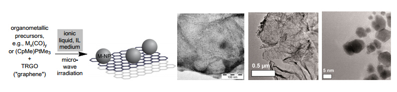
Marquardt D, Vollmer C, Thomann R, et al. (2011) The use of microwave irradiation for the easy synthesis of graphene-supported transition metal hybrid nanoparticles in ionic liquids. Carbon 49: 1326-1332. doi: 10.1016/j.carbon.2010.09.066
    [32] Marquardt D, Beckert F, Pennetreau F, et al. (2014) Hybrid materials of platinum nanoparticles and thiol-functionalized graphene derivatives. Carbon 66: 285-294. doi: 10.1016/j.carbon.2013.09.002
    [33] Mingos DMP, Baghurst DR, (1991) Applications of microwave dielectric heating effects to synthetic problems in chemistry. Chem Soc Rev 20: 1-47. doi: 10.1039/cs9912000001
    [34] Galema SA, (1997) Microwave chemistry. Chem Soc Rev 26: 233-238. doi: 10.1039/cs9972600233
    [35] Larhed M, Moberg C, Hallberg A, (2002) Microwave-accelerated homogeneous catalysis in organic chemistry. Acc Chem Res 35: 717-727. doi: 10.1021/ar010074v
    [36] Bilecka I, Niederberger M, (2010) Microwave chemistry for inorganic nanomaterials synthesis. Nanoscale 2: 1358-1374. doi: 10.1039/b9nr00377k
    [37] Leonelli C, Mason, TJ, (2010) Microwave and ultrasonic processing: Now a realistic option for industry. Chem. Engineering and Processing 49: 885-900. doi: 10.1016/j.cep.2010.05.006
  • Reader Comments
  • © 2014 the Author(s), licensee AIMS Press. This is an open access article distributed under the terms of the Creative Commons Attribution License (http://creativecommons.org/licenses/by/4.0)
通讯作者: 陈斌, bchen63@163.com
  • 1. 

    沈阳化工大学材料科学与工程学院 沈阳 110142

  1. 本站搜索
  2. 百度学术搜索
  3. 万方数据库搜索
  4. CNKI搜索

Metrics

Article views(6012) PDF downloads(1147) Cited by(8)

Other Articles By Authors

/

DownLoad:  Full-Size Img  PowerPoint
Return
Return

Catalog