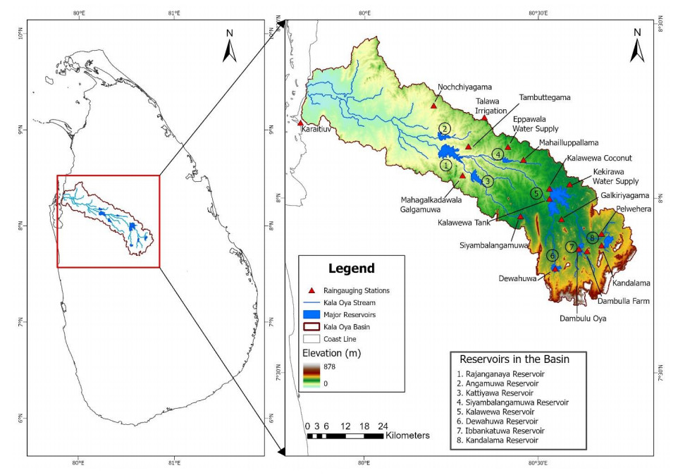
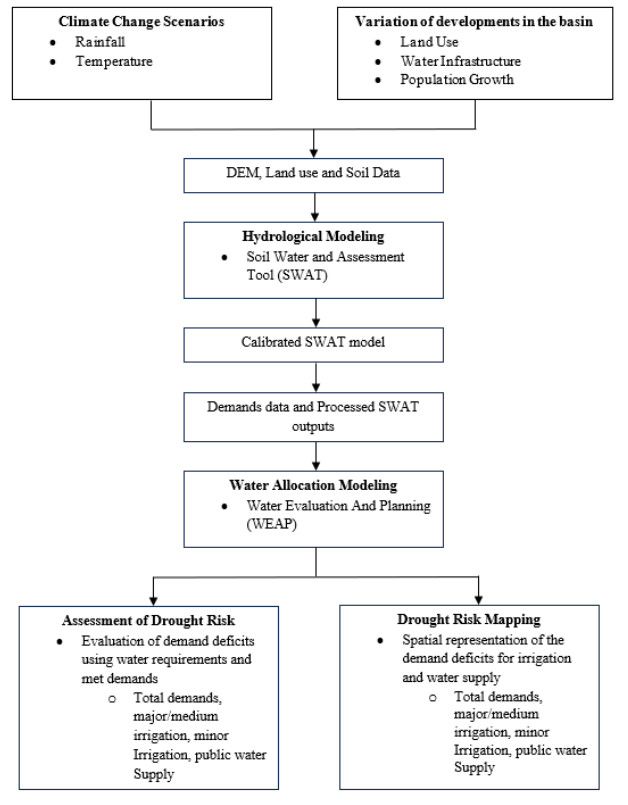
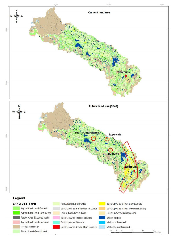
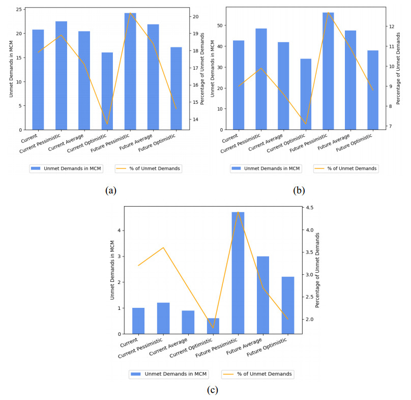
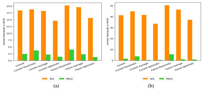
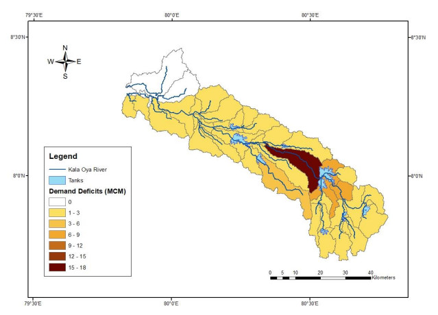
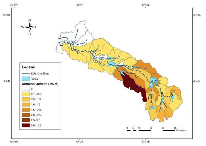
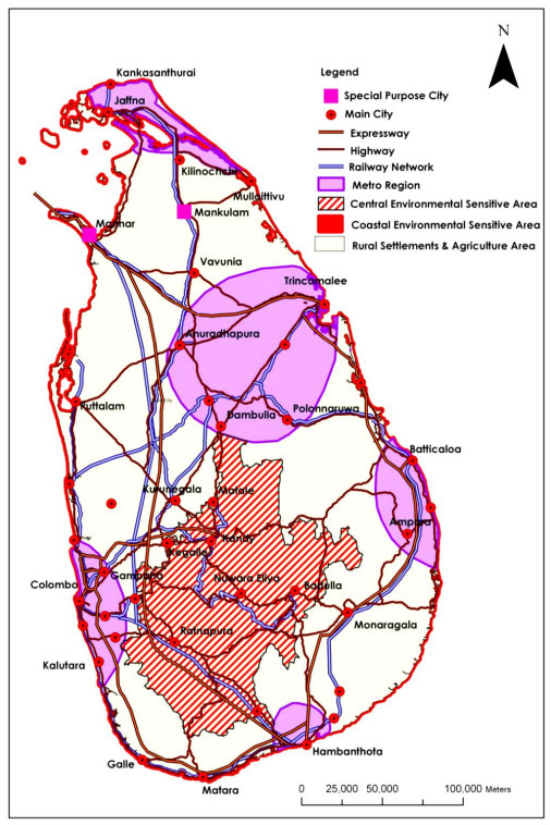
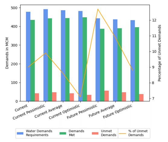
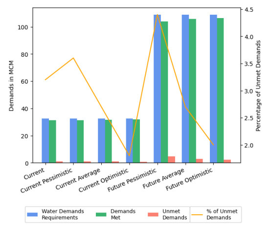
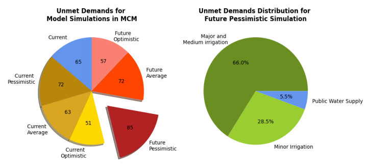
Kala Oya is one of the drier river basins in Sri Lanka that is affected by droughts for certain time periods. Water shortages are visible in crop yields and public water supply due to climate change. Consequently, the Soil and Water Assessment Tool (SWAT) was used to develop hydrological models, and Water Evaluation and Planning (WEAP) software was used to analyze the water allocation for the basin. The software's evaluation and assessing capability of allocation of water, transmission, and diversion links for demands are some reasons to use WEAP as a separate water allocation model. The future land use and climate aspect (2040) has also been included in these models to enable the generation of "scenarios" that can be used to test the demand deficits for irrigation and public water supply. Three climatic conditions such as optimistic, pessimistic, and average for 2040 were considered for modeling. Our major findings include: 1. The pessimistic climate change scenario exhibits the highest rise in drought metrics while the optimistic represents the lowest. Under current land use conditions, annual Long-Term Average (LTA) public water supply deficits are 1.0 million cubic meters (MCM) (3.2%), and for future land use, in a pessimistic climate change scenario, annual LTA deficits are 4.7 MCM (4.4%). 2. For medium/major irrigated agriculture, annual LTA deficits for current conditions are 42.8 MCM (9.0%), and for future land use, pessimistic climate change scenarios are 56.1 MCM (12.7%). For minor irrigation, annual LTA deficits for current conditions are 20.8 MCM (17.9%) and future pessimistic climate change scenarios are 24.2 MCM (20.2%). 3. This study concludes that the public water supply demand deficits are considerably greater in the middle and lower catchments of Kala Oya basin for future land use (with basin developments) model simulations. This may create water scarcity and social stress for people who require immediate mitigation measures. 4. Overall, it was revealed that the agriculture-oriented drought losses (major/medium irrigation) are significant (around 66–67% of total demand deficits) in the Kala Oya basin, and they may create adverse impacts on the country's economy due to crop yield losses.
Citation: Sajana Pramudith Hemakumara, Thilini Kaushalya, Kamal Laksiri, Miyuru B Gunathilake, Hazi Md Azamathulla, Upaka Rathnayake. Incorporation of SWAT & WEAP models for analysis of water demand deficits in the Kala Oya River Basin in Sri Lanka: perspective for climate and land change[J]. AIMS Geosciences, 2025, 11(1): 155-200. doi: 10.3934/geosci.2025008
Kala Oya is one of the drier river basins in Sri Lanka that is affected by droughts for certain time periods. Water shortages are visible in crop yields and public water supply due to climate change. Consequently, the Soil and Water Assessment Tool (SWAT) was used to develop hydrological models, and Water Evaluation and Planning (WEAP) software was used to analyze the water allocation for the basin. The software's evaluation and assessing capability of allocation of water, transmission, and diversion links for demands are some reasons to use WEAP as a separate water allocation model. The future land use and climate aspect (2040) has also been included in these models to enable the generation of "scenarios" that can be used to test the demand deficits for irrigation and public water supply. Three climatic conditions such as optimistic, pessimistic, and average for 2040 were considered for modeling. Our major findings include: 1. The pessimistic climate change scenario exhibits the highest rise in drought metrics while the optimistic represents the lowest. Under current land use conditions, annual Long-Term Average (LTA) public water supply deficits are 1.0 million cubic meters (MCM) (3.2%), and for future land use, in a pessimistic climate change scenario, annual LTA deficits are 4.7 MCM (4.4%). 2. For medium/major irrigated agriculture, annual LTA deficits for current conditions are 42.8 MCM (9.0%), and for future land use, pessimistic climate change scenarios are 56.1 MCM (12.7%). For minor irrigation, annual LTA deficits for current conditions are 20.8 MCM (17.9%) and future pessimistic climate change scenarios are 24.2 MCM (20.2%). 3. This study concludes that the public water supply demand deficits are considerably greater in the middle and lower catchments of Kala Oya basin for future land use (with basin developments) model simulations. This may create water scarcity and social stress for people who require immediate mitigation measures. 4. Overall, it was revealed that the agriculture-oriented drought losses (major/medium irrigation) are significant (around 66–67% of total demand deficits) in the Kala Oya basin, and they may create adverse impacts on the country's economy due to crop yield losses.

| [1] | Nairizi S (2017) Irrigated Agriculture Development under Drought and Water Scarcity. International Commission on Irrigation and Drainage: New Delhi, India. Available from: https://www.icid.org/drought_pub2017.pdf. |
| [2] | UN-Water, Summary Progress Update 2021: SDG 6—water and sanitation for all, 2021. Available from: https://www.unwater.org/sites/default/files/app/uploads/2021/12/SDG-6-Summary-Progress-Update-2021_Version-July-2021a.pdf. |
| [3] | Unnicef, Water Scarcity, 2021. Available from: https://www.unicef.org/wash/water-scarcity. |
| [4] | Intergovernmental Panel on Climate Change, Climate Change, Synthesis Report, 2023,184. https://doi.org/10.59327/IPCC/AR6-9789291691647 |
| [5] |
Rosenzweig C, Tubiello FN, Tubiello R, et al. (2002) Increased crop damage in the US from excess precipitation under climate change. Global Environ Change 12: 197–202. https://doi.org/10.1016/S0959-3780(02)00008-0 doi: 10.1016/S0959-3780(02)00008-0

|
| [6] |
Yadav P, Jaiswal DK, Sinha RK (2021) Climate change: Impact on agricultural production and sustainable mitigation. Global Clim Change, 151–174. https://doi.org/10.1016/B978-0-12-822928-6.00010-1 doi: 10.1016/B978-0-12-822928-6.00010-1
|
| [7] |
Trenberth KE (2018) Climate change caused by human activities is happening and it already has major consequences. J Energy Nat Resour Law 36: 463–481. https://doi.org/10.1080/02646811.2018.1450895 doi: 10.1080/02646811.2018.1450895
|
| [8] |
Zubair L (2003) El Niño–southern oscillation influences on the Mahaweli streamflow in Sri Lanka. Int J Climatol J R Meteorol Soc 23: 91–102. https://doi.org/10.1002/joc.865 doi: 10.1002/joc.865
|
| [9] |
Domroes M (1979) Monsoon and land use in Sri Lanka. Geojournal 3: 179–192. https://doi.org/10.1007/BF00257707 doi: 10.1007/BF00257707
|
| [10] |
Ranatunge E, Malmgren BA, Hayashi Y, et al. (2003) Changes in the Southwest Monsoon mean daily rainfall intensity in Sri Lanka: relationship to the El Niño–Southern Oscillation. Palaeogeogr Palaeoclimatol Palaeoecol 197: 1–14. https://doi.org/10.1016/S0031-0182(03)00383-3 doi: 10.1016/S0031-0182(03)00383-3
|
| [11] |
Rathnayake U (2019) Comparison of statistical methods to graphical methods in rainfall trend analysis: case studies from tropical catchments. Adv Meteorol 2019: 1–10. https://doi.org/10.1155/2019/8603586 doi: 10.1155/2019/8603586
|
| [12] | Yoshino MM, Suppiah R (1984) Rainfall and paddy production in Sri Lanka. J Agric Meteorol 40: 9–20. https://www.jstage.jst.go.jp/article/agrmet1943/40/1/40_1_9/_article/-char/ja/ |
| [13] |
Prasanna RPIR (2018) Economic costs of drought and farmers' adaptation strategies: Evidence from Sri Lanka. Sri Lanka J Econ Res 5: 61–79. https://doi.org/10.4038/sljer.v5i2.49 doi: 10.4038/sljer.v5i2.49
|
| [14] | Disaster Management Centre, Drought Situation Report—Sri Lanka, Ministry of Public Administration and Disaster Management: Colombo, 2018. Available from: https://www.dmc.gov.lk/index.php?lang = en |
| [15] |
Geekiyanage N, Pushpakumara DKNG (2013) Ecology of ancient tank cascade systems in island Sri Lanka. J Mar Isl Cult 2: 93–101. https://doi.org/10.1016/j.imic.2013.11.001 doi: 10.1016/j.imic.2013.11.001
|
| [16] |
Perera KARS, Amarasinghe MD (2019) Carbon sequestration capacity of mangrove soils in micro tidal estuaries and lagoons: A case study from Sri Lanka. Geoderma 347: 80–89. https://doi.org/10.1016/j.geoderma.2019.03.041 doi: 10.1016/j.geoderma.2019.03.041
|
| [17] |
Krysanova V, White M (2015) Advances in water resources assessment with SWAT—an overview. Hydrol Sci J 60: 771–783. https://doi.org/10.1080/02626667.2015.1029482 doi: 10.1080/02626667.2015.1029482
|
| [18] |
Makumbura RK, Gunathilake MB, Samarasinghe JT, et al. (2022) Comparison of Calibration Approaches of the Soil and Water Assessment Tool (SWAT) Model in a Tropical Watershed. Hydrology 9: 183. https://doi.org/10.3390/hydrology9100183 doi: 10.3390/hydrology9100183
|
| [19] |
Shelton S (2021) Evaluation of the Streamflow Simulation by SWAT Model for Selected Catchments in Mahaweli River Basin, Sri Lanka. Water Conserv Sci Eng 6: 233–248. https://doi.org/10.1007/s41101-021-00117-w doi: 10.1007/s41101-021-00117-w
|
| [20] |
Krysanova V, Arnold JG (2008) Advances in ecohydrological modelling with SWAT—a review. Hydrol Sci J 53: 939–947. https://doi.org/10.1623/hysj.53.5.939 doi: 10.1623/hysj.53.5.939
|
| [21] |
Cloke HL, Pappenberger F (2009) Ensemble flood forecasting: A review. J Hydrol 375: 613–626. https://doi.org/10.1016/j.jhydrol.2009.06.005. doi: 10.1016/j.jhydrol.2009.06.005
|
| [22] |
Mohammed K, Islam AKMS, Islam GMT, et al. (2017) Impact of High-End Climate Change on Floods and Low Flows of the Brahmaputra River. J Hydrol Eng 22: 04017041. https://doi.org/10.1061/(ASCE)HE.1943-5584.0001567 doi: 10.1061/(ASCE)HE.1943-5584.0001567
|
| [23] |
McDaniel RL, Munster C, Nielsen-Gammon J (2017) Crop and location specific agricultural drought quantification: part Ⅲ. Forecasting water stress and yield trends. Trans ASABE 60: 741–752. https://doi.org/10.13031/trans.11651 doi: 10.13031/trans.11651
|
| [24] |
Chathuranika IM, Gunathilake MB, Baddewela PK, et al. (2022) Comparison of Two Hydrological Models, HEC-HMS and SWAT in Runoff Estimation: Application to Huai Bang Sai Tropical Watershed, Thailand. Fluids 7: 267. https://doi.org/10.3390/fluids7080267 doi: 10.3390/fluids7080267
|
| [25] |
Meehl GA, Covey C, Delworth T, et al. (2007) THE WCRP CMIP3 Multimodel Dataset: A New Era in Climate Change Research. Bull Am Meteorol Soc 88: 1383–1394. https://doi.org/10.1175/BAMS-88-9-1383 doi: 10.1175/BAMS-88-9-1383
|
| [26] |
Arabi M, Frankenberger JR, Engel BA, et al. (2008) Representation of agricultural conservation practices with SWAT. Hydrol Processes 22: 3042–3055. https://doi.org/10.1002/hyp.6890 doi: 10.1002/hyp.6890
|
| [27] |
Fohrer N, Haverkamp S, Eckhardt K, et al. (2001) Hydrologic response to land use changes on the catchment scale. Phys Chem Earth Part B Hydrol Oceans Atmos 26: 577–582. https://doi.org/10.1016/S1464-1909(01)00052-1 doi: 10.1016/S1464-1909(01)00052-1
|
| [28] |
Li Z, Liu WZ, Zhang XC, et al. (2009) Impacts of land use change and climate variability on hydrology in an agricultural catchment on the Loess Plateau of China. J Hydrol 377: 35–42. https://doi.org/10.1016/j.jhydrol.2009.08.007 doi: 10.1016/j.jhydrol.2009.08.007
|
| [29] |
Lin S, Jing C, Chaplot V, et al. (2010) Effect of DEM resolution on SWAT outputs of runoff, sediment and nutrients. Hydrol Earth Syst Sci Discuss 7: 4411–4435. https://doi.org/10.5194/hessd-7-4411-2010 doi: 10.5194/hessd-7-4411-2010
|
| [30] |
Park JY, Park MJ, Ahn SR, et al. (2011) Assessment of future climate change impacts on water quantity and quality for a mountainous dam watershed using SWAT. Trans ASABE 54: 1725–1737. https://doi.org/10.13031/2013.39843 doi: 10.13031/2013.39843
|
| [31] |
Yates D, Sieber J, Purkey D, et al. (2005) WEAP21—A Demand-, Priority-, and Preference-Driven Water Planning Model: Part 1: Model Characteristics. Water Int 30: 487–500. https://doi.org/10.1080/02508060508691893 doi: 10.1080/02508060508691893
|
| [32] |
Lévite H, Sally H, Cour J (2003) Testing water demand management scenarios in a water-stressed basin in South Africa: application of the WEAP model. Phys Chem Earth Parts A/B/C 28: 779–786. https://doi.org/10.1016/j.pce.2003.08.025 doi: 10.1016/j.pce.2003.08.025
|
| [33] |
Amin A, Iqbal J, Asghar A, et al. (2018) Analysis of Current and Future Water Demands in the Upper Indus Basin under IPCC Climate and Socio-Economic Scenarios Using a Hydro-Economic WEAP Model. Water 10: 537. https://doi.org/10.3390/w10050537 doi: 10.3390/w10050537
|
| [34] |
Abbas SA, Xuan Y, Bailey RT (2022) Assessing Climate Change Impact on Water Resources in Water Demand Scenarios Using SWAT-MODFLOW-WEAP. Hydrology 9: 164. https://doi.org/10.3390/hydrology9100164 doi: 10.3390/hydrology9100164
|
| [35] |
Hamza AA, Getahun BA (2022) Assessment of water resource and forecasting water demand using WEAP model in Beles river, Abbay river basin, Ethiopia. Sustain. Water Resour Manag 8: 22. https://doi.org/10.1007/s40899-022-00615-2 doi: 10.1007/s40899-022-00615-2
|
| [36] |
Dlamini N, Senzanje A, Mabhaudhi T (2023) Assessing climate change impacts on surface water availability using the WEAP model: A case study of the Buffalo River catchment, South Africa. J Hydrol Reg Stud 46: 101330. https://doi.org/10.1016/j.ejrh.2023.101330 doi: 10.1016/j.ejrh.2023.101330
|
| [37] |
Moghadam SH, Ashofteh PS, Loáiciga HA (2022) Optimal Water Allocation of Surface and Ground Water Resources Under Climate Change with WEAP and IWOA Modeling. Water Resour Manag 36: 3181–3205. https://doi.org/10.1007/s11269-022-03195-0 doi: 10.1007/s11269-022-03195-0
|
| [38] | Opere AO, Waswa R, Mutua FM (2022) Assessing the impacts of climate change on surface water resources using WEAP model in Narok county, Kenya. Front Water 3: 789340. |
| [39] |
Kishiwa P, Nobert J, Kongo V, et al. (2018) Assessment of impacts of climate change on surface water availability using coupled SWAT and WEAP models: case of upper Pangani River Basin, Tanzania. Proc IAHS 378: 23–27. https://doi.org/10.5194/piahs-378-23-2018 doi: 10.5194/piahs-378-23-2018
|
| [40] |
Goyburo A, Rau P, Lavado-Casimiro W, et al. (2023) Assessment of Present and Future Water Security under Anthropogenic and Climate Changes Using WEAP Model in the Vilcanota-Urubamba Catchment, Cusco, Perú. Water 15: 1439. https://doi.org/10.3390/w15071439 doi: 10.3390/w15071439
|
| [41] |
Touseef M, Chen L, Yang W (2021) Assessment of Surface Water Availability under Climate Change Using Coupled SWAT-WEAP in Hongshui River Basin, China. ISPRS Int J Geo-Inf 10: 298. https://doi.org/10.3390/ijgi10050298 doi: 10.3390/ijgi10050298
|
| [42] | Kaushalya RDT, Hemakumara SP (2020) Integration of SWAT and WEAP Models for Water Resource Management in the Malwathu Oya Basin, Sri Lanka. Resilient dams for future. Colombo: Sri Lanka National Committee on Large Dams (SLNCOLD) Bulletin. |
| [43] | Climate Change Secretariat, National adaptation plan for climate change impacts in Sri Lanka: 2016–2025. Colombo, Sri Lanka, 2016. Available from: https://eohfs.health.gov.lk/environmental/images/pdf/downloads/NAP-For-Sri-Lanka_2016-2025.pdf. |
| [44] | Iresh ADS (2023) Drought studies in Kala Oya basin, Sri Lanka. Water Prod J 3: 19–34. |
| [45] | Weerasinghe KD, Zubair L (2013) Farmer & river basin management, policy perspectives on adapting to climate variability & climate Change in north western Sri Lanka. |
| [46] |
Iresh ADS, Marasingha AGNS, Wedanda AMTSH, et al. (2021) Development of a Hydrological Model for Kala Oya Basin Using SWAT Model. Eng J Inst Eng Sri L 54: 57–65. https://doi.org/10.4038/engineer.v54i1.7435 doi: 10.4038/engineer.v54i1.7435
|
| [47] | Department of Census and Statistics, Census of Population and Housing 2012, Battaramulla: Department of Census and Statistics, 2015. Available from: http://www.statistics.gov.lk/Resource/en/Population/CPH_2011/CPH_2012_5Per_Rpt.pdf. |
| [48] | River basin planning & management division, Final Interim report on Comprehensive Plan for Kala Oya Basin, Colombo: Mahaweli Authority of Sri Lanka, 2003. Available from: https://mahaweli.gov.lk/about%20us.html. |
| [49] | Perera HDBS, Vidanage SP, Kallesoe MF (2005) Multiple Benefits of Small Irrigation Tanks and Their Economic Value: A Case Study in the Kala Oya Basin, Sri Lanka, IUCN-The World Conservation Union, Sri Lanka Country Office. |
| [50] |
Lloyd-Hughes B, Saunders MA (2002) A drought climatology for Europe. Int J Climatol 22: 1571–1592. https://doi.org/10.1002/joc.846 doi: 10.1002/joc.846
|
| [51] | CGIAR, MarkSimGCM: Weather Generating Tool, 2013. Available from: https://ccafs.cgiar.org/resources/tools/marksimgcm-weather-generating-tool. |
| [52] | CGIAR, MarkSimTM GCM—DSSAT weather file generator, 2010. Available from: https://gisweb.ciat.cgiar.org/MarksimGCM/docs/doc.html. |
| [53] |
Hargreaves GH, Allen RG (2003) History and evaluation of Hargreaves evapotranspiration equation. J Irrig Drain Eng 129: 53–63. https://doi.org/10.1061/(ASCE)0733-9437(2003)129:1(53) doi: 10.1061/(ASCE)0733-9437(2003)129:1(53)
|
| [54] | National Physical Planning Policy and Plan Sri Lanka, Battaramulla: National Physical Planning Department (NPPD), 2010. |
| [55] | Ministry of Water Supply, National Water Supply & Drainage Board Coporate Plan 2020–2025. Colombo: National Water & Drainage Board (NWSDB). 2020. Available from: https://www.waterboard.lk/publications/ |
| [56] | Vidanage S, Perera S, Kallesoe MF (2005) The value of traditional water schemes: Small tanks in the Kala Oya Basin, Sri Lanka, 6. IUCN. |
| [57] | Ministry of Irrigation and Water Resources Management, Dam safety and water resources planning project (DSWRPP) Operation and maintenance manual Kalawewa Dam. 2012. Available from: https://www.irrigation.gov.lk/web/index.php?lang = en. |
| [58] |
Alahacoon N, Amarnath G (2022) Agricultural drought monitoring in Sri Lanka using multisource satellite data. Adv Space Res 69: 4078–4097. https://doi.org/10.1016/j.asr.2022.03.009 doi: 10.1016/j.asr.2022.03.009
|


Figures(22) / Tables(31)

Sajana Pramudith Hemakumara, Thilini Kaushalya, Kamal Laksiri, Miyuru B Gunathilake, Hazi Md Azamathulla, Upaka Rathnayake. Incorporation of SWAT & WEAP models for analysis of water demand deficits in the Kala Oya River Basin in Sri Lanka: perspective for climate and land change[J]. AIMS Geosciences, 2025, 11(1): 155-200. doi: 10.3934/geosci.2025008


 DownLoad: