Educational thematic mapping of cultural &amp; natural heritage in southern Italy during and after the COVID-19 pandemic

Francesco De Pascale; Giuseppe Ferraro; Francesco De Pascale; Giuseppe Ferraro

doi:10.3934/geosci.2022037

AIMS Geosciences

2022, Volume 8, Issue 4: 669-685. doi: 10.3934/geosci.2022037

Previous Article Next Article

Research article Special Issues

Educational thematic mapping of cultural & natural heritage in southern Italy during and after the COVID-19 pandemic

Francesco De Pascale ^{1
,
,},
Giuseppe Ferraro ²

1.
Department of Culture and Society, University of Palermo, 90128 Palermo, Italy
2.
Director of the Institute for the History of the Italian Risorgimento, Provincial Committee of Cosenza, Italy

Received: 31 July 2022 Revised: 11 September 2022 Accepted: 25 September 2022 Published: 09 October 2022

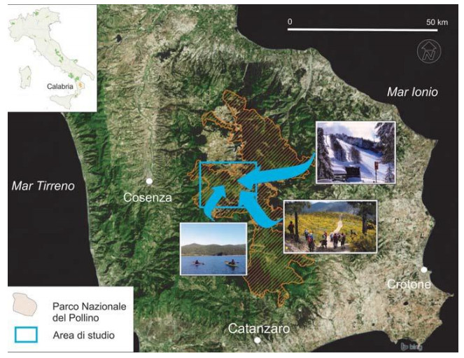
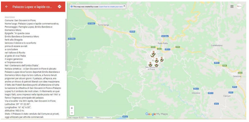
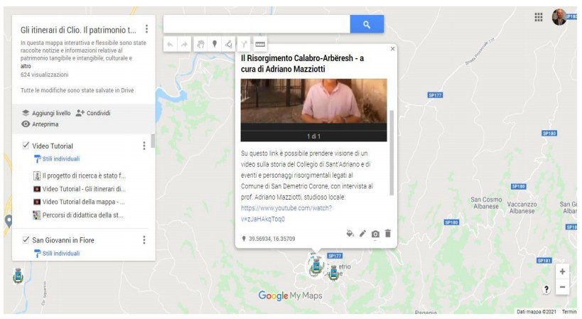
This paper will describe the creation of an interactive and flexible map through which news and information relating to the tangible and intangible cultural and natural heritage of the Sila National Park area (Calabria, southern Italy, related to the Italian Risorgimento period) were collected. The map, which can be updated daily, can be accessed by clicking on a location's reference. The pop-up window contains information for each character, monument, commemorative plaque and palace linked to the history of the Risorgimento. Anthropological and oral traditions linked to the affected area are also listed. The map is enriched by a focus on significant archaeological presences, characters and productive activities linked to the Risorgimento or our present time. Each pop-up is also characterized by the possibility of viewing any photographs and historical documentation, as well as research videos and educational and informative material. This paper's research questions concern 1) how the thematic map on Google Maps can be useful for educational purposes and 2) how the map was used to enhance the cultural and natural heritage of the Sila National Park and to promote an ethics-based tourism during and after the pandemic. The historical-geographical itinerary of the map, therefore, offers hints and suggestions for sustainable cultural tourism initiatives open to international context and proximity. Neogeographic technologies such as Google Maps have been used because they facilitate and stimulate the sharing and production of geographic information. In the case of this map, it was created from a bottom-up approach that involved local stakeholders and scholars.
- banditry,
- Covid-19 pandemic,
- education,
- heritage,
- Risorgimento,
- Sila National Park (Southern Italy),
- thematic map,
- virtual tourism
Citation: Francesco De Pascale, Giuseppe Ferraro. Educational thematic mapping of cultural & natural heritage in southern Italy during and after the COVID-19 pandemic[J]. AIMS Geosciences, 2022, 8(4): 669-685. doi: 10.3934/geosci.2022037

Related Papers:

Abstract

This paper will describe the creation of an interactive and flexible map through which news and information relating to the tangible and intangible cultural and natural heritage of the Sila National Park area (Calabria, southern Italy, related to the Italian Risorgimento period) were collected. The map, which can be updated daily, can be accessed by clicking on a location's reference. The pop-up window contains information for each character, monument, commemorative plaque and palace linked to the history of the Risorgimento. Anthropological and oral traditions linked to the affected area are also listed. The map is enriched by a focus on significant archaeological presences, characters and productive activities linked to the Risorgimento or our present time. Each pop-up is also characterized by the possibility of viewing any photographs and historical documentation, as well as research videos and educational and informative material. This paper's research questions concern 1) how the thematic map on Google Maps can be useful for educational purposes and 2) how the map was used to enhance the cultural and natural heritage of the Sila National Park and to promote an ethics-based tourism during and after the pandemic. The historical-geographical itinerary of the map, therefore, offers hints and suggestions for sustainable cultural tourism initiatives open to international context and proximity. Neogeographic technologies such as Google Maps have been used because they facilitate and stimulate the sharing and production of geographic information. In the case of this map, it was created from a bottom-up approach that involved local stakeholders and scholars.

References

[1]	Papadakis S, Trampas A, Barianos A, et al. (2020) Evaluating the Learning Process: The "ThimelEdu" Educational Game Case Study. Proc 12th Int Conf Comput Supported Educ 2: 290–298. https://doi.org/10.5220/0009379902900298 doi: 10.5220/0009379902900298
[2]	Papadakis S, Kalogiannakis M, Sifaki E, et al. (2018) Access Moodle Using Smart Mobile Phones. A Case Study in a Greek University. Interactivity Game Creat Des Learn Innovation 229: 376–385. https://doi.org/10.1007/978-3-319-76908-0_36 doi: 10.1007/978-3-319-76908-0_36
[3]	Dalelovna Shakirova N, Al Said N, Mihailovna Konyushenko S (2020) The Use of Virtual Reality in Geo-Education. Int J Emerging Technol Learn 20: 59–70.
[4]	Caldis S (2019) Geography and STEM. Geogr Educ 32: 5–10.
[5]	De Pietro O, De Pascale F (2020) STEAM educational paths to fight the educational poverty and reduce the disaster risk: an experimental activity in a primary school. J Education Technol Soc Stud 12: 167–191.
[6]	De Pascale F (2018) Percorsi interdisciplinari STEAM per la scuola del futuro. Ambiente Società Territorio. Geografia Nelle Scuole 3: 38–42.
[7]	De Pascale F (2020) Un itinerario geostorico virtuale su Google Maps, percepito e rappresentato da bambini di scuola primaria, a 160 anni dall'Unità d'Italia. Rivista calabrese di Storia del '900 1–2: 97–110.
[8]	Dorouka P, Papadakis S, Kalogiannakis M (2020) Tablets and apps for promoting robotics, mathematics, STEM education and literacy in early childhood education. Int J Mobile Learn Organ 4: 255–274. https://doi.org/10.1504/IJMLO.2020.106179 doi: 10.1504/IJMLO.2020.106179
[9]	Costantino D, Angelini MG, Alfio VS, et al. (2020) Implementation of a System WebGIS Open-Source for the Protection and Sustainable Management of Rural Heritage. Appl Geomat 12: 41–54. https://doi.org/10.1007/s12518-019-00275-6 doi: 10.1007/s12518-019-00275-6
[10]	Tommasi A, Cefalo R, Zardini F, et al. (2017) Using Webgis and Cloud Tools to Promote Cultural Heritage Dissemination: The Historic up Project. Int Arch Photogramm Remote Sens Spatial Inf Sci 42: 663–668. https://doi.org/10.5194/isprs-archives-XLII-5-W1-663-2017 doi: 10.5194/isprs-archives-XLII-5-W1-663-2017
[11]	Suma A, de Cosmo P (2011) Geodiv Interface: An Open Source Tool For Management And Promotion Of The Geodiversity Of Sirra De Grazalema Natural Park (Andalusia, Spain). GeoJournal Tourism Geosites 8: 309–318.
[12]	Lerario A, Maiellaro N, Zonno M (2010) Remote Fruition of Architectures: R & D and Training Experiences. Proc 2010 Second Int Conf Adv Multimedia 49–54. https://doi.org/10.1109/MMEDIA.2010.38 doi: 10.1109/MMEDIA.2010.38
[13]	Santos CADJ, Campos AC, Rodrigues LP (2019) GIS and Touristic Itineraries. The Case of São Cristóvão, Sergipe, Brazil. Cad De Geogr 39: 29–39. https://doi.org/10.14195/0871-1623_39_3 doi: 10.14195/0871-1623_39_3
[14]	Cayla N, Hoblea F, Gasquet D (2009) Place de La Géomorphologie Dans l'offre Géotouristique de l'arc Alpin: Du Réel Au Virtuel. Géomorphosites 65–71.
[15]	Luppichini M, Noti V, Pavone D, et al. (2022) Web Mapping and Real–Virtual Itineraries to Promote Feasible Archaeological and Environmental Tourism in Versilia (Italy). ISPRS Int J Geo-Inf 11: 460. https://doi.org/10.3390/ijgi11090460 doi: 10.3390/ijgi11090460
[16]	Weng YH, Sun FS, Grigsby JD (2012) GeoTools: An Android Phone Application in Geology. Comput Geosci 44: 24–30. https://doi.org/10.1016/j.cageo.2012.02.027 doi: 10.1016/j.cageo.2012.02.027
[17]	Sâvulescu I, Mihai B (2011) Mapping Forest Landscape Change in Iezer Mountains, Romanian Carpathians. AGIS Approach Based on Cartographic Heritage, Forestry Data and Remote Sensing Imagery. J Maps 7: 429–446.
[18]	Coscarelli R, Antronico L, De Pascale F, et al. (2021) Turismo, Paesaggio e Beni Culturali. Prospettive di tutela, valorizzazione e sviluppo sostenibile. Quaderni della Società Italiana di Scienze del Turismo, 275–292.
[19]	Regional Tourism Observatory of the Calabria Region, Calabria Tourism, 2022. Available from: https://osservatoriointernazionalizzazione.regione.calabria.it/.
[20]	UNESCO, Sila, Commissione Nazionale Italiana per l'UNESCO, Roma, 2020. Available from: http://www.unesco.it/it/RiserveBiosfera/Detail/92.
[21]	LENA G, PAGANO M (2019) Clima e popolamento umano in Sila Grande durante il primo millennio. Geol Tec Ambientale 1: 57–65.
[22]	Sila National Park, Geography, 2018. Available from: https://www.parcosila.it/it/la-natura/geografia.html.
[23]	Cappelli V (2021) I laghi della Sila. La grande trasformazione dell'altopiano silano. Stratigrafie del Paesaggio 2: 37–53.
[24]	Placanica A (1985) I caratteri originali, in BEVILACQUA P. e PLACANICA A, Eds., La Calabria. Storia d'Italia. Le Regioni dall'Unità a oggi, Einaudi, Torino, 3–114.
[25]	Bernardo M, De Pascale F (2017) Le vie della transumanza in Calabria: un itinerario culturale percepito tra geostoria, economia e letteratura. La Dea Editori, Camigliatello Silano.
[26]	Molfese F (1964) Storia del brigantaggio dopo l'Unità. Istituto Gramsci, 781–794.
[27]	Pinto C (2019) La guerra per il Mezzogiorno. Italiani, borbonici e briganti 1860–1870, by Carmine Pinto, Bari-Roma, Editori Laterza, 2019,496 pp., € 23.85 (hardback), ISBN 978-88-581-3531-0. Mod Italy 25: 101–103. https://doi.org/10.1017/mit.2019.58. doi: 10.1017/mit.2019.58
[28]	Gaudioso F (1987) Calabria ribelle. Brigantaggio e sistemi repressivi nel Cosentino (1860–1870). FrancoAngeli, Milano.
[29]	Scirocco A (1991) Briganti e società nell'Ottocento. Il caso Calabria, Capone Editore, Lecce.
[30]	Ferraro G (2016) Il prefetto e i briganti. La Calabria e l'unificazione italiana (1861–1865), Le Monnier, Firenze.
[31]	Galasso G (1975) Economia e società nella Calabria del Cinquecento, Feltrinelli, Milano.
[32]	Isnardi G (1965) Stranieri e italiani in Calabria nell'800 e nel primo '900. Frontiera calabrese Napoli, 368–369.
[33]	Placanica A (2001) Il Medioevo: la terra e gli uomini. Storia della Calabria, Laterza, Roma-Bari, 56–75.
[34]	Placanica A (2001) L'immagine della Calabria: realtà e fortuna di uno stereotipo. Storia della Calabria, Laterza, Roma-Bari, 88–107.
[35]	Ferraro G, De Pascale F, Mastroianni D (2021) Parco Nazionale della Sila. Mappa tematica con Google Maps. Il Quotidiano del Sud, 33.
[36]	Goodchild MF, Glennon JA (2010) Crowdsourcing geographic information for disaster response: a research frontier. Int J Digital Earth 3: 231–241. https://doi.org/10.1080/17538941003759255. doi: 10.1080/17538941003759255
[37]	De Pascale F (2021) Paesaggi nei mondi virtuali e neogeografia. "Il mio spazio vissuto": una mappatura delle testimonianze di quarantena durante il lockdown in Italia. Configurazioni e trasfigurazioni. Discorsi sul paesaggio mediato, Nuova Trauben, Turin, 145–158.
[38]	De Pascale F, Travis C (2022) The COVID-19 Testimonies Map: Representing Italian "Pandemic Space" Perceptions with Neogeography Technologies. Routledge Handbook of the Digital Environmental Humanities, Routledge, London, 419–427.
[39]	Padula V (1980) Il Bruzio, Gangemi, Roma.
[40]	Ferraro G (2021), Didattica e storia del Risorgimento. Pratiche, metodi e suggerimenti per le scuole secondarie di secondo grado. Didattica Della Storia Journal of Research and Didactics of History 3: 114–133. https://doi.org/10.6092/issn.2704-8217/12537 doi: 10.6092/issn.2704-8217/12537
[41]	Adorno S (2020) Pensare la didattica della storia, Pensare storicamente. Didattica, laboratori, manuali, FrancoAngeli, Milano, 11–28.
[42]	Marangi M (2016) In "media" res. Adolescenti e media contemporanei. Nuova Secondaria 9: 36–39.
[43]	De Luna G (1994) L'occhio e l'orecchio dello storico. Le fonti audiovisive nella ricerca e nella didattica della storia, La Nuova Italia, Firenze.
[44]	De Luna G (2001) La passione e la ragione. Fonti e metodi dello storico contemporaneo, La Nuova Italia, Milano.
[45]	Corrao P, Viola P (2005). Introduzione agli studi di storia, Donzelli, Roma.
[46]	Gambi L (1973) Una geografia per la storia. Einaudi, Torino.
[47]	Rocca G (2011) Il sapere geografico tra ricerca e didattica: basi concettuali, strumenti e progettazione di percorsi didattici, Pàtron, Bologna.
[48]	Pepe P (2019) Dalla classe di concorso 39/A alla classe A21. Le azioni dell'AIIG. Dal riordino 2010 in poi. Ambiente Società Territorio. Geografie nelle scuole, 3.
[49]	Istituto Calabrese per la Storia dell'Antifascismo e dell'Italia Contemporanea, Smurra, Tiberio, 2022. Available from: https://www.icsaicstoria.it/smurra-tiberio.
[50]	WTTC, Travel & Tourism. Global Economic Impact & Trends, 2021. Available from: https://wttc.org/Research/Economic-Impact.
[51]	Rajamanicam H, Mohanty P, Chandran A (2018) Assessing the responsible tourism practices for sustainable development—An empirical inquiry of yelagiri, Tamil Nadu. Johar 13: 1–29.
[52]	UNWTO, UNWTO World Tourism Barometer, Madrid, Spain, 2020. Available from: https://www.e-unwto.org/loi/wtobarometereng.
[53]	Ndou V, Mele G, Hysa E, et al. (2022) Exploiting Technology to Deal with the COVID-19 Challenges in Travel & Tourism: A Bibliometric Analysis. Sustainability 14: 5917. https://doi.org/10.3390/su14105917 doi: 10.3390/su14105917
[54]	Oncioiu I, Priescu I (2022), The Use of Virtual Reality in Tourism Destinations as a Tool to Develop Tourist Behavior Perspective. Sustainability 14: 4191. https://doi.org/10.3390/su14074191 doi: 10.3390/su14074191
[55]	UNWTO, 'Overtourism'? Understanding and Managing Urban Tourism Growth beyond Perceptions: Executive Summary, 2018. Available from: https://www.e-unwto.org/doi/book/10.18111/9789284420070.
[56]	United Nations, The 2030 Agenda for Sustainable Development: the 17 Goals, 2015. Available from: https://sdgs.un.org/goals.
[57]	De Pascale F (2017) Geoethics and Sustainability Education Through an Open Source CIGIS Application: the Memory of Places Project in Calabria, Southern Italy, as a Case Study, Going beyond sustainability in Heritage Studies No 2, Springer Heritage Studies, 295–306.
[58]	Bernardo M, De Pascale F (2019) A Study on Memory Sites Perception in Primary School for Promoting the Urban Sustainability Education: A Learning Module in Calabria (Southern Italy). Sustainability 11: 6379. https://doi.org/10.3390/su11226379 doi: 10.3390/su11226379

Reader Comments

Your name:*

Email:*
© 2022 the Author(s), licensee AIMS Press. This is an open access article distributed under the terms of the Creative Commons Attribution License (http://creativecommons.org/licenses/by/4.0)