Citation: Kazuhisa A. Chikita. Environmental factors controlling stream water temperature in a forest catchment[J]. AIMS Geosciences, 2018, 4(4): 192-214. doi: 10.3934/geosci.2018.4.192
| [1] | Quentin Fiacre Togbévi, Luc Ollivier Sintondji . Hydrological response to land use and land cover changes in a tropical West African catchment (Couffo, Benin). AIMS Geosciences, 2021, 7(3): 338-354. doi: 10.3934/geosci.2021021 |
| [2] | Jennifer B Alford, Jose A Mora . Factors influencing chronic semi-arid headwater stream impairments: a southern California case study. AIMS Geosciences, 2022, 8(1): 98-126. doi: 10.3934/geosci.2022007 |
| [3] | Rafael Gotardo, Gustavo A. Piazza, Edson Torres, Vander Kaufmann, Adilson Pinheiro . Soil Loss Vulnerability in an Agricultural Catchment in the Atlantic Forest Biome in Southern Brazil. AIMS Geosciences, 2016, 2(4): 345-365. doi: 10.3934/geosci.2016.4.345 |
| [4] | Eric Ariel L. Salas, Sakthi Subburayalu Kumaran, Robert Bennett, Leeoria P. Willis, Kayla Mitchell . Machine Learning-Based Classification of Small-Sized Wetlands Using Sentinel-2 Images. AIMS Geosciences, 2024, 10(1): 62-79. doi: 10.3934/geosci.2024005 |
| [5] | Adeeba Ayaz, Maddu Rajesh, Shailesh Kumar Singh, Shaik Rehana . Estimation of reference evapotranspiration using machine learning models with limited data. AIMS Geosciences, 2021, 7(3): 268-290. doi: 10.3934/geosci.2021016 |
| [6] | John Greenway . Water resources management versus the world. AIMS Geosciences, 2021, 7(4): 589-604. doi: 10.3934/geosci.2021035 |
| [7] | Alessia Nannoni, Federica Meloni, Marco Benvenuti, Jacopo Cabassi, Francesco Ciani, Pilario Costagliola, Silvia Fornasaro, Pierfranco Lattanzi, Marta Lazzaroni, Barbara Nisi, Guia Morelli, Valentina Rimondi, Orlando Vaselli . Environmental impact of past Hg mining activities in the Monte Amiata district, Italy: A summary of recent studies. AIMS Geosciences, 2022, 8(4): 525-551. doi: 10.3934/geosci.2022029 |
| [8] | Dek Vimean Pheakdey, Tran Dang Xuan, Tran Dang Khanh . Influence of Climate Factors on Rice Yields in Cambodia. AIMS Geosciences, 2017, 3(4): 561-575. doi: 10.3934/geosci.2017.4.561 |
| [9] | Sajana Pramudith Hemakumara, Thilini Kaushalya, Kamal Laksiri, Miyuru B Gunathilake, Hazi Md Azamathulla, Upaka Rathnayake . Incorporation of SWAT & WEAP models for analysis of water demand deficits in the Kala Oya River Basin in Sri Lanka: perspective for climate and land change. AIMS Geosciences, 2025, 11(1): 155-200. doi: 10.3934/geosci.2025008 |
| [10] | Maurizio Barbieri, Tiziano Boschetti, Giuseppe Sappa, Francesca Andrei . Hydrogeochemistry and groundwater quality assessment in a municipal solid waste landfill (central Italy). AIMS Geosciences, 2022, 8(3): 467-487. doi: 10.3934/geosci.2022026 |
The change of stream water temperature could produce several physical, chemical and biological activities [1], and sensitively affect the ecosystem in streams, lakes or estuarine coastal regions. By estimating the heat budget of some rivers in England, Webb and Zhang [2,3] revealed that the thermal system of rivers differs depending on the basin scale, seasons and groundwater input. Moore et al. [4] pointed out that a hyporheic heat exchange in the heat budget tends to reduce the increase of stream water temperature in a headwater region by deforestation.
A few studies about the stream heat budget were conducted in forest and open streams [5,6]. They estimated the stream heat budget through one season, and discussed the mechanism of change of water temperature in a forest stream. Nakamura and Dokai [7] and Sugimoto et al. [8] estimated the stream heat budget in the summer season. However, there are few studies about the heat budget of a stream in a completely forested catchment for a period longer than one season. In order to investigate the mechanism of water temperature change in such a stream, it is necessary to estimate the stream heat budget throughout the pre-foliation, foliation and defoliation periods. Moore et al. [4] pointed out that the hemispherical photography can quantify radiative fluxes above a stream. Dugdale et al. [9] revealed that the net heat flux at stream surface and stream water temperature vary greatly by riparian vegetation types. In this study, stream heat budget along the channels is estimated by quantifying shades above the stream in pre-foliation, foliation and defoliation periods, and the stream water temperature is simulated by using the estimated heat budget.
In order to investigate stream water temperature in a forest region, the Putoisaroma Stream, Hokkaido, Japan, was chosen as a typical forest stream (Figure 1). The stream is a tributary of the Saromabetsu River flowing into brackish Lake Saroma, connected to the Sea of Okhotsk. The stream basin (43° 54'N, 143° 38'E) has the drainage area of 19.0 km2 and the altitude of 137 m a.s.l. at site P1 (7.8 km2 and 189 m a.s.l. at site P3). The climatic condition of the Saromabetsu River basin is sub-frigid and humid with annual mean air temperature of 5.4 ℃ and mean annual precipitation of 813 mm in 1999–2008. The monthly mean air temperature ranges from -9.2 ℃ in January to 19.7 ℃ in August. The peak monthly precipitation is 135 mm in August. These data are referred to the Automated Meteorological Data Acquisition System (AMeDAS) at the Saroma town, about 15 km northeast of site P1. The stream basin upstream of site P3 is completely covered by the mixed deciduous and coniferous forests (e.g. Larix kaempferi, Abies sachalinensis, Betula platyphylla var. japonica), while the stream basin between sites P1 and P3 is occupied mostly by grasslands and fields. The basin geology consists of the alluvial deposit in or around the stream channels between sites P1 and P2, the Yubetsu Group bedrock (pebbly sandstone, sandstone and shale) around sites P3 and P4, and the mixture of the Saroma Group bedrock (shale) and the Nikoro Group bedrock (greenstone, breccia, sandstone and shale) around sites P5, P6 and P7. The Yubetsu Group bedrock and the Saroma Group bedrock are dated from the Cretaceous to Paleogene, while the Nikoro Group bedrock belongs to the Jurassic to Cretaceous [10]. The streambed materials are mainly composed of non-vegetated gravels and coarse sands overlying the bedrocks.
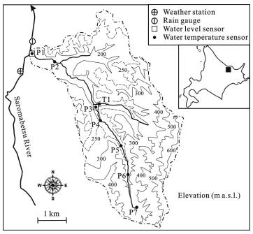 Figure 1. Location of the Putoisaroma stream catchment, Hokkaido, Japan, and observation sites in the catchment.
Meteorological conditions were monitored at the weather station in an open field 1 km south of site P1 in June 2008 to October 2009 (Figure 1), and simultaneously measured above the stream about once per month. The weather station monitored shortwave radiation, air temperature, relative humidity, wind velocity and atmospheric pressure at 10 min intervals. Temperature data loggers (StowAway TidbiT, Onset Computer Corporation, USA; accuracy of ±0.2 ℃) were set at site P1 and sites P3 to P7 and buried at depths of 5 cm and 30 cm below the streambed of site P3 to monitor stream water temperature and streambed temperature at intervals of 30 min, respectively. Water level was measured at sites P1 and P3 at intervals of 30 min. A piezometer, which consists of a water level sensor and a stainless steel pipe of 32 mm diameter and 910 mm in length, was set in the mid-channel of site P3 to monitor groundwater level at intervals of 1 hr, whereby the influence of groundwater inflow or outflow and associated heat flux were considered. A steel pipe with a 24-mesh net and a water level sensor at the bottom was then fixed at a depth of 25 cm below the streambed. Using the piezometer, a hydraulic test by the Baxter method [11] was carried out to obtain the saturated hydraulic conductivity of streambed. Subsequently the vertical flux of water infiltrating the streambed at site P3 was calculated by applying the Darcy's law to differences between the stream stage and piezometer's level.
The meteorology above the stream was observed at all the observation sites about once per month. We then measured air temperature, relative humidity and wind velocity five times at the interval of 1 minute, using a portable weather meter (Kestrel 4500 Pocket Weather Tracker, Nielsen-Kellerman, USA). The observed data were compared with the data of the weather station to know how meteorological conditions in the open field are different from those in the forest. The discharge measurements and topographic surveys across the channels were simultaneously conducted.
In order to quantify the shades at stream surface, hemispherical photographs were taken at about 70 cm above stream surface at the observation sites at intervals of about 1 month, using a fisheye lens (Gyorome 8, Flexible Image Technology, Japan) attached to a compact digital camera (Optio M10, PENTAX, Japan). The shading factor (SF: the quantified shade above the stream) was computed from hemispherical photographs by using the Gap Light Analyzer [12] with 10° resolution for both azimuthal and zenithal angles. The Gap Light Analyzer tends to overestimate the shaded area, since all the leaves are judged to have the black shade in spite of the incomplete opacity of broad leaves for the shortwave radiation. The weather data in the snowfall season of November 2008 to mid May 2009 were provided by the AMeDAS at the Saroma town.
The stream heat budget is estimated to investigate how hydrological and meteorological parameters affect the stream water temperature. Considering Eq 1 of the energy balance and Eq 2 of the water budget in each stream reach of site P7 to site P3 (Figure 1), advective heat flux, non-advective heat flux and water temperature are calculated by Eq 3:
| cwρwwLydTwdt=cwρwQusTus+cwρwQgwTgw+cwρwQpTp+wLHnet−cwρwQdsTds | (1) |
| Qds=Qus+Qgw+Qp | (2) |
| Twn+1=Twn+Δtcwρwy[Hnet+cwρwQdswL(Tus−Tds)+cwρwQgwwL(Tgw−Tus)+cwρwQpwL(Tp−Tus)] | (3) |
where cw is specific heat of water (J kg-1 ℃-1), ρw is water density (kg m-3), w is stream width (m), L is stream length (m) between the upstream end and downstream end, y is mean water depth (m), Twn is water temperature (℃) at a time n, Qus is upstream discharge (m3 s-1), Tus is upstream water temperature (℃), Qgw is groundwater inflow in a reach (m3 s-1), Tgw is groundwater temperature (℃), Qp is precipitation input (m3 s-1) over stream surface, Tp is precipitation temperature (℃), Hnet is non-advective net heat flux (W m-2), Qds is downstream discharge (m3 s-1), and Tds is downstream water temperature (℃). The cw and ρw values, depending on water temperature, were obtained as those for the mean values of measured water temperature by using empirical formulae in Kell [13]. Stream water temperature and all the heat flux terms were calculated at intervals of 1 hr (i.e., the time step Δt = 3600 s), using hourly or hourly mean hydrological and meteorological data.
Three advective heat fluxes related to downstream discharge Qds, groundwater inflow Qgw and precipitation input Qp are included in the bracket on the right side of Eq 3. The first term is due to advective cool (or warm) water input from upstream, which is a function of both downstream discharge Qds and stream temperature differences between the upstream site and the downstream site. The second term is the advection by groundwater input from streambed. Groundwater discharge Qgw was calculated from discharge differences between the upstream site and the downstream site on non-rainfall days. Groundwater temperature Tgw was assumed to be equal to stream temperature at site P7, where discharge is mostly influenced by groundwater. The third term is the advection due to precipitation input over stream surface. Precipitation discharge Qp was calculated from precipitation Pr (m s-1) multiplied by stream width w and reach length L. Precipitation temperature Tp was assumed to be equal to air temperature at the time because the wet-bulb temperature is nearly equal to the air temperature during rainfalls. Here, we exclude the intervals when intermittent rains occur or the time when a rain starts, because of no validity of the assumption.
The non-advective net heat flux Hnet in Eq 3 consists of two heat exchanges, heat exchange Hsurf (W m-2) at water surface and heat exchange Hbed (W m-2) at streambed as follows:
| Hnet=Hsurf+Hbed | (4) |
Heat exchange Hsurf has four types of heat exchange as shown by Eq 5, while Hbed has two types of heat exchange as in Eq 6:
| Hsurf=K∗+L∗+He+Hs | (5) |
| Hbed=Hbc+Hbf | (6) |
where K* is net shortwave radiation (W m-2), L* is net longwave radiation (W m-2), He is evaporative heat flux (W m-2), Hs is sensible heat flux (W m-2), Hbc is streambed heat conduction (W m-2), and Hbf is streambed friction (W m-2). Each heat flux is positive when the heat transfers from atmosphere or streambed to stream water. In Eq 5, He and Hs values are positive under condition of condensation and air temperature higher than stream water temperature, respectively [14].
The net shortwave radiation K* is shown by Eq 7:
| K∗=(1−SF)(1−α)K↓ | (7) |
where SF is the shading factor calculated by the Gap Light Analyzer, α is albedo at stream surface ( = 0.05), and K↓ is incoming shortwave radiation (W m-2) monitored at the weather station. The α value of 0.05 was adopted as a typical value for mountain streams [15], though the albedo becomes relatively high under the turbid water during high stream discharge. The net longwave radiation L* is separated into the incoming longwave radiation from both atmosphere and riparian objects (i.e., surrounding slope and vegetation) to stream water, and the outgoing longwave radiation emitted from stream water to both atmosphere and riparian objects. Here, the incoming longwave radiation from riparian objects to stream water was assumed to be equal in magnitude to the outgoing longwave radiation from stream water to riparian objects, because the emissivities of riparian objects and stream water are almost equal at 0.95 to 0.97. Here, it is assumed that the topography around the stream does not give any significant contribution to the determination of radiative fluxes at stream surface. The net longwave radiation is thus shown by Eq 8:
| L∗=(1−SF)L↓net+(1−SF)L↑=(1−SF)(1−α)εaσ(Ta+273.2)4+[−(1−SF)εwσ(Tw+273.2)4] | (8) |
where L↓net is net incoming longwave radiation (W m-2) emitted from atmosphere to stream water, L↑ is outgoing longwave radiation (W m-2) emitted from stream water to atmosphere, εa is atmospheric emissivity, σ is the Stefan-Boltzmann constant (5.67 × 10⁻⁸ W m-2 ℃-4), Ta is air temperature (℃), εw is stream water emissivity ( = 0.95), and Tw is stream water temperature (℃). Here, the albedo for the longwave radiation is assumed to be equal to that for the shortwave radiation [16]. Morin and Couillard [17] expressed the atmospheric emissivity εa by the following:
| εa=0.74+0.0087ea(1+0.17C2) | (9) |
where ea is air water vapor pressure (hPa) and C is cloud cover (from 0 at clear sky to 1 at wholly cloudy sky).
Using the bulk method, evaporative heat flux He and sensible heat flux Hs are expressed as follows:
| He=lρaηCEpaV(ea−ew) | (10) |
| Hs=cpρaCHV(Ta−Tw) | (11) |
where l is latent heat (J kg-1) for vaporization, ρa is air density (kg m-3), η is molecular-weight ratio of water vapor to dry air ( = 0.622), CE and CH are bulk transfer coefficients ( = 1.20 × 10⁻³), pa is atmospheric pressure (hPa), V is wind velocity (m s-1) at 2 m above water surface, and ew is saturated vapor pressure (hPa) at stream surface temperature. The vapor pressure ew is calculated using the Tetens' equation [18]. For the application of Eqs 10 and 11, the log law of wind velocity is assumed to be valid along the relatively straight river channels (Figure 1).
Streambed heat conduction Hbc is calculated using the following Fourier's law:
| Hbc=KbTb30−Tb05Δz | (12) |
where Kb is thermal conductivity ( = 2.6 W m-1 ℃-1) of streambed materials, Tb30 and Tb05 are streambed temperature (℃) at 30 cm and 5 cm in depth, respectively, Δz is the distance ( = 0.25 m) between two streambed temperature sensors. Streambed friction Hbf is calculated by the following equation [19]:
| Hbf=ρwgQwI | (13) |
where g is gravitational acceleration ( = 9.8 m s-2), Q is stream discharge (m3 s-1), and I is mean streambed slope.
The advective and non-advective heat fluxes were calculated at site P3, and then the observed water temperature time series at site P3 were simulated by using Eq 3. The heat flux Hsurf at stream surface was calculated at each of sites P1, P3, P5, P6 and P7, in order to know how the stream heat exchange changes spatially.
Figure 2 shows temporal variations of daily mean stream water temperature at sites P1, P3 to P7 and T1, daily mean streambed temperature at site P3, daily mean air temperature by the AMeDAS at the Saroma town, daily mean stream discharge at sites P1 and P3, and diurnal precipitation at near site P1 in July 2008 to October 2009. The daily mean temperature for air, stream water and streambed varied seasonally. The daily mean air temperature ranged from about -10 ℃ in January and February to about 20 ℃ in July and August. Meanwhile, the daily mean stream water and streambed temperatures ranged from 0 ℃ in December–March to about 15 ℃ in July–August. The daily mean stream discharge was about 0.05 m3 s-1 in the winter (December to February with daily mean air temperature of about 0 ℃ or less) and during non-rainfalls. The stream discharge exceeded 1 m3 s-1 when snowmelt and heavy rainfalls occurred in April and in May to October, respectively.
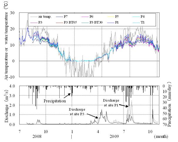 Figure 2. Temporal variations of air temperature by the AMeDAS at the Saroma town, stream water temperature at sites P1, P3 to P7 and T1, streambed temperature at site P3 and stream discharge at sites P1 and P3, and diurnal precipitation near site P1 in July 2008 to October 2009. The labels, P3 BT05 and P3 BT30, indicate the streambed temperature at depths of 5 cm and 30 cm below the streambed at site P3, respectively.
Figure 3 shows temporal variations of the vertical water flux through streambed, the stream stage, the piezometer's level and the head loss at site P3 for 19 June–27 August 2009. The stream stage is consistently higher than the piezometer's level, and thus the head loss (i.e., stream level minus groundwater level) is always positive. This indicates that the stream water output through streambed occurred at site P3. Using the head loss of less than 0.05 m and the saturated hydraulic conductivity of 0.119 m s-1, the specific discharge ranged from 0 to 3 × 10⁻⁴ m s-1. The stream water output at site P3 is thus very small.
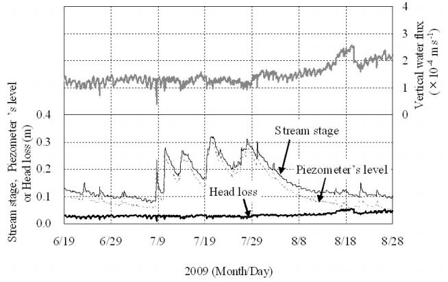 Figure 3. Temporal variations of hourly mean vertical water flux, stream stage, piezometer's level and head loss at site P3 for 19 June–27 August 2009. The head loss is equal to the stream stage minus piezometer's level.
Figure 4 shows typical daily variations of hourly mean stream water temperature and streambed temperature in 2009. The daily variation of stream water temperature for 19–22 May is relatively great in amplitude (Figure 4a), which is about 4 ℃ at site P7 and about 8 ℃ at site P1. The streambed temperature then exceeded the stream water temperature over the night, but lower than the stream water temperature on the daytime. The relatively small variation of stream water temperature occurred in June (Figure 4b), indicating the amplitudes of about 1℃ at site P7 and about 4 ℃ at site P1. The streambed temperature at 30 cm below streambed was then consistently lower than the stream water temperature at sites P1, P3 and P5. Both stream water temperature and streambed temperature hardly varied in late July (Figure 4c). In October, the daily variation of stream water temperature was small with the amplitudes of about 2℃ at site P7 and about 3 ℃ at site P1 (Figure 4d). The streambed temperature was then similar to or higher than the water temperature.
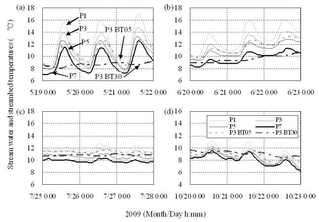 Figure 4. Temporal variations of hourly mean stream water temperature at sites P1, P3, P5 and P7 and hourly mean streambed temperature (BT05 and BT30) at site P3 for (a) 19–22 May, (b) 20–23 June, (c) 25–28 July and (d) 20–23 October 2009.
As a result, the stream water receives much heat on the daytimes of May and June (Figure 4a, b), but on the night, loses most of the heat in May and little in June. Thus, the stream water temperature in May increased drastically from the morning to noon, and then decreased rapidly down to below the streambed temperature until the next early morning. Stream water temperature in June changed more moderately day after day. Unusually long rainfalls occurred in July 2009 (Figure 2). The stream water then seems to have conducted quite a small heat exchange due to the low solar radiation (Figure 4c). In October, the stream water seems to have received little heat on daytime due to the low solar radiation and the low air temperature, and to have lost the heat on the night due to the nocturnal cooling (Figure 4d).
Figure 5 shows a temporal change of stream water temperature between site P7 and site P1 (a) at 2 hr or 4 hr intervals for 24 hrs in May and October of 2009 ((a) 0600h to 1400h, 20 May, (b) 1400h, 20 May to 0600h, 21 May, (c) 0600h to 1400h, 21 October, and (d) 1400h, 21 October to 0600h, 22 October. The stream water temperature in May increases linearly along the stream channels, while, in October, it hardly increases. The maximum and minimum of the increments between sites P1 and P7 were 4.6 ℃/(7425 m) on 20 May (Figure 5a) and 1.6 ℃/(7425 m) on 21 October (Figure 5c), respectively. This indicates that, in May, the advection of relatively cool water from the upstream occurred more strongly than in October.
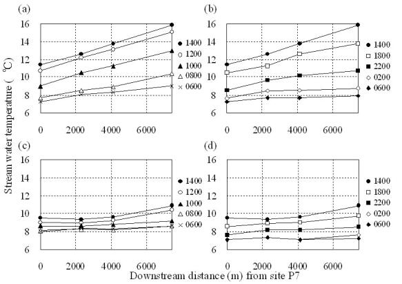 Figure 5. Temporal changes of stream water temperature at site P7 (distance, 0 m), site P5 (2300m), site P3 (4125m) and site P1 (7425 m) for 24 hours in May and October of 2009. (a) 0600h to 1400h, 20 May, (b) for 1400h, 20 May to 0600h, 21 May, (c) for 0600h to 1400h, 21 October, and (d) for 1400h, 21 October 21 to 0600h, 22 October.
Figure 6 shows a downstream change of the ratio of stream discharge at each of sites P4, P5, P6 and P7 to the discharge at site P3 during non-rainfalls. Except for the P5–P4 reach in May 2009, the discharge increased by about 70% of the P3 discharge between site P7 and site P5 (distance, 2300 m), and by about 30 % of the P3 discharge between site P5 and site P3 (distance, 4125 m). This indicates that the groundwater input between sites P5 and P3 is relatively very small. The decrease of discharge in the P5–P4 reach in May 2009 is possibly due to the stream water output into groundwater in the plain downstream of site P5 by the increased stream stage from snowmelt (Figures 1 and 2). At site P3, the stream water output through the streambed slightly occurred as shown by the records of the piezometer's level and stream stage in Figure 3.
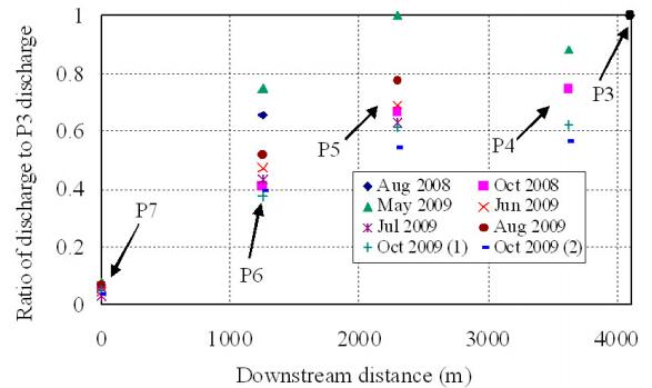 Figure 6. Downstream change of the ratio of stream discharge at site P7 (0 m), site P6 (1250 m), site P5 (2300 m) and site P4 (3750 m) to that at site P3 (4125 m) in each month of 2008 and 2009.
It is necessary to consider meteorological conditions above the stream when the weather station is far from the stream. Benyahya et al. [6] concluded that the air temperature, relative humidity and wind velocity above the stream are slightly lower, a little higher and below one third smaller than those in the open field, respectively. The comparison of meteorological conditions between the Putoisaroma stream and the weather station in the open field indicates that air temperature and relative humidity are hardly different, but that wind speed is relatively very low above the stream (Figure 7). The ratio of air temperature (i.e., mean air temperature above the stream divided by the mean air temperature at the weather station) was 101.2% with the high correlation (R2 = 0.882) between air temperature above the stream and that at the weather station. The ratio of relative humidity was 99.5% with R2 = 0.775, while the ratio of wind speed was 28.4% with R2 = 0.348. Thus, the air temperature and relative humidity above the stream were nearly equal to those at the weather station, but the wind speed above the stream was less than one third as large as that at the weather station. The low wind speed above the stream is produced by surrounding hill slopes, lateral stream banks and vegetation to obstruct the wind pathways. In particular, at the most upstream site P7, the wind speed was about one fifth as high as that at the weather station. Meanwhile, the wind direction above the stream was distributed roughly along the stream channels. Thus, the stream channel itself could be a main wind pathway, and the wind speed above stream surface may follow the log law of wind velocity.
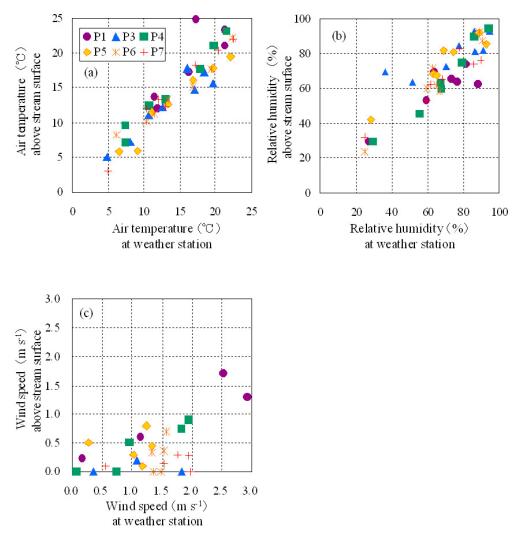 Figure 7. Relations between the meteorological conditions above stream surface and those at the weather station. (a) Air temperature, (b) relative humidity and (c) wind speed.
Hemispherical photographs and calculated shading factors at sites P1, P3, P4 and P7 in May–October 2009 are shown in Figure 8 to Figure 10. The shading factors (SF = 0.015 to 0.059) at site P1 are consistently smaller than those (SF = 0.125–0.870) at sites P3 to P7 in the forest region. Site P4 is located in the relatively open area with riparian young spruce (Figure 1), thus indicating the shading factor of less than 0.5 even during the foliation period. The hemispherical photographs at sites P3, P4 and P7 indicate that the riparian trees give the relatively large shade at the stream surface. At the most upstream site P7, the surrounding slopes also give the large shaded area.
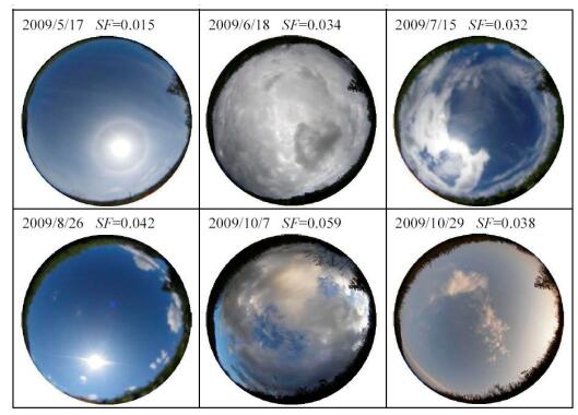 Figure 8. Hemispherical photographs and calculated shading factors, SF, at site P1.
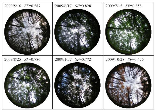 Figure 9. Hemispherical photographs and calculated shading factors, SF, at site P3.
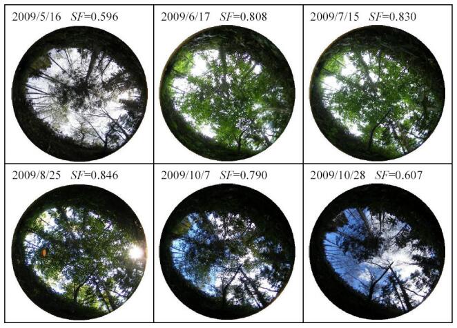 Figure 10. Hemispherical photographs and calculated shading factors, SF, at site P7.
The shading factors were numerically obtained in May to October 2009 (Figure 11). The pre-foliation and defoliation appear before mid-May and after late October, respectively. The shading factors in forest (sites P3, P5, P6 and P7) ranged from 0.466 to 0.611 on 16 May, from 0.711 to 0.870 on 17 June to 7 October, and from 0.192 to 0.607 on 28 October. As a result, the foliation and defoliation cause the shading factors to seasonally change. The seasonal and spatial changes of the shading factors suggest that the shaded area at stream surface was successfully quantified in space and time. This result is useful to investigate which thermal factors control stream water temperature.
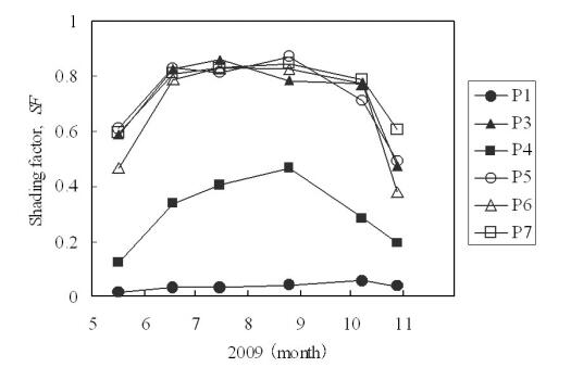 Figure 11. Seasonal change of the shading factor at each site in 2009.
Figure 12 shows temporal variations of daily mean non-advective heat fluxes at site P3 in 2009. The non-advective heat fluxes consist of (a) net shortwave radiation and net longwave radiation, (b) evaporative heat flux, (c) sensible heat flux, (d) streambed heat conduction, and (e) streambed friction. The net shortwave radiation acts as a major heat source, while the net longwave radiation and streambed heat conduction work as major heat losses (Figure 12a, d). The daily mean net shortwave radiation ranged from 1.6 W m-2 to 116.2 W m-2 with the average of 29.1 W m-2. Meanwhile, the daily mean net longwave radiation ranged from -33.5 W m-2 to 4.8 W m-2 with the average of -7.6 W m-2. The streambed heat conduction takes the average of -8.7 W m-2, especially indicating a very low value for 18 May - 9 July 2009 (-14.8 W m-2 on average) (Figure 12d).
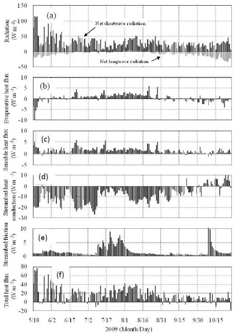 Figure 12. Temporal variations of daily mean non-advective heat fluxes at site P3 in 2009. (a) Net shortwave radiation and net longwave radiation, (b) evaporative heat flux, (c) sensible heat flux, (d) streambed heat conduction, (e) streambed friction, and (f) total non-advective heat flux.
The magnitudes of the evaporative and sensible heat fluxes and the streambed friction are smaller than those of the radiative fluxes and streambed heat conduction (Figure 12b, c, e). The evaporative heat flux ranges from -10.1 W m-2 to 6.0 W m-2 with the average of 0.3 W m-2. The sensible heat flux ranges from -1.5 W m-2 to 5.8 W m-2 with the average of 1.4 W m-2. The streambed friction ranges from 0.4 W m-2 to 17.6 W m-2 with the average of 1.7 W m-2. It is thus seen that these three heat fluxes hardly influence stream water temperature. For the heat exchange Hsurf at water surface in Eq 5, in this study, evaporative and sensible heat fluxes on the stream bank and catchment slope around the stream channel are neglected, in addition to the radiative fluxes. No consideration of the topographic effects on the energy balance could underestimate stream water temperature, if it is numerically simulated.
The net shortwave radiation reached to the maximum in mid-May, gradually decreased until late June, and hardly changed in late June to October. The net longwave radiation worked as a heat loss in May to mid-July and in mid-August to October, but as a heat source in mid-July to mid-August. It attained to the minimum in late October.
Both the shading factor and solar radiation are considered to influence the seasonal change of the incoming shortwave radiation into the stream. The high incoming shortwave radiation at stream surface in May is barely obstructed by the riparian vegetation, because of the pre-foliation and the low shading factor. During the foliation (i.e. after mid-June), the incoming shortwave radiation is clearly obstructed by the riparian vegetation, although the solar radiation is relatively strong between the summer solstice (21 June) and autumnal equinox (23 September). This is why the net shortwave radiation is low after mid-June. In the defoliation period, when the shading factor decreases, the incoming shortwave radiation is scarcely obstructed as in the pre-foliation period. However, the net shortwave radiation then keeps low, because the solar radiation is weakened through the season. The net shortwave radiation thus keeps low also for the post-defoliation period after late October
The shading factor and the air temperature mainly influence the seasonal change of the longwave radiation. The magnitude of the net longwave radiation decreases with increasing shading factor for the periods of pre-foliation to foliation, and then increases with decreasing shading factor for the periods of foliation to defoliation. In general the shade tends to obstruct both the incoming shortwave radiation and the exchange of the longwave radiation between atmosphere and stream water. The minimum net longwave radiation in late October is due to the radiative cooling from the low shading factor and low air temperature. The low shading factor produces the high exchange of the longwave radiation, while the low air temperature decreases the incoming longwave radiation from atmosphere to stream surface. The coupled thermal conditions seem to have produced the lowest net longwave radiation.
The seasonal change of the evaporative heat flux is seen (Figure 12b). The evaporative heat flux was negative (i.e., evaporation) in May, September and October, but positive (i.e., condensation) in June to August. In May, September and October, the daily mean air temperature was almost consistently higher than the daily mean water temperature (Figure 2). The streambed heat conduction also seasonally varied (Figure 12d). The streambed heat conduction was negative (cooling the stream water) in May to September, but positive (heating the stream water) in October. The seasonal fluctuation of the streambed temperature is smaller than that of the stream water temperature (Figures 2 and 4). Thus, the streambed tends to repeat the heat input to stream water and the heat loss from stream water.
The total non-advective heat fluxes are almost positive (Figure 12f). The stream water temperature can thus continue to increase if the stream water was influenced only by the non-advective heat fluxes. However, the stream water temperature decreased in August to October (Figure 2). This is because the advective heat fluxes also strongly influence the stream water temperature even for the low discharge period.
Figure 13 shows diurnal variation of each stream heat flux at site P3 (a) on a fine day (19 May 2009) in the pre-foliation period, (b) on a fine day (26 August 2009) in the foliation period, (c) on a fine day (25 October 2009) in the post-defoliation period, and (d) on a rainy day (19 July 2009) in the foliation period. Here, the "fine days" are defined as days with sunshine hours nearly equal to the potential sunshine hours at both the weather stations in the open filed and the Saroma town. On the fine days (Figure 13a, b, c), the net shortwave radiation and net incoming longwave radiation are main heat sources to the stream, while the outgoing longwave radiation and advective heat flux from upstream are main heat losses from the stream. On the rain day (Figure 13d), both the heat sources and heat losses are relatively small at less than 60 W m-2 in magnitude. Then, the net incoming longwave radiation and the advective heat flux from upstream (AU) act as main heat sources, while the outgoing longwave radiation and the advective heat flux by groundwater (AG) work as main heat losses. The AU acted temporarily as a heat loss, when the discharge peaked at 15:00 on 19 July. It is noted that, on the rainy day, both AU and AG exhibit relatively large fluctuations. The streambed heat conduction acted as a heat loss in the summer (Figure 13a, b, d) and as a heat source in the autumn (Figure 13c). The other fluxes (evaporative heat flux, sensible heat flux, streambed friction, advective heat flux by groundwater and advective heat flux by precipitation) indicate the daily variations but with the very small magnitude.
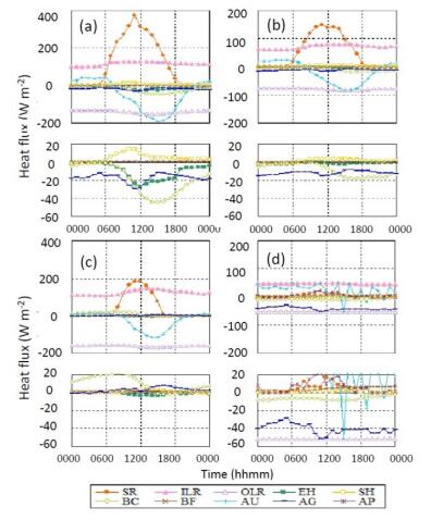 Figure 13. Diurnal variation of each stream heat flux at site P3 in 2009. (a) Fine day (19 May) in the pre-foliation period, (b) fine day (26 August) in the foliation period, (c) fine day (25 October) in the post-defoliation period and (d) rainy day (19 July) in the foliation period. SR: net shortwave radiation, ILR: net incoming longwave radiation, OLR: outgoing longwave radiation, EH: evaporative heat flux, SH: sensible heat flux, BC: streambed heat conduction, BF: streambed friction, AU: advective heat flux from upstream, AG: advective heat flux by groundwater, AP: advective heat flux by precipitation.
On the daytime of 19 May, the net shortwave radiation (SR) acted as the relatively very large heat source (Figure 13a). This results from the large solar radiation and low shading factor in the pre-foliation period. Subsequently the advective heat flux from upstream (AU) worked as one of the large heat losses on the afternoon. The large spatial change of stream water temperature in May (Figure 4a, b) likely produced the large advective heat flux from upstream. The net shortwave radiation on 26 August was lower than on 19 May (Figure 13b). The increased shading factor by foliation probably decreased the net shortwave radiation, although the incoming solar radiation in the open field decreased from May to August. The magnitudes of the net incoming longwave radiation and the outgoing longwave radiation also decreased on 26 August. Hence, the shading factor seems to decrease not only the net shortwave radiation but also the incoming and outgoing longwave radiations.
The net incoming longwave radiation and the outgoing longwave radiation increase their magnitude on 25 October (Figure 13c), compared to that on 26 August (Figure 13b). Especially the outgoing longwave radiation became the largest heat loss of stream water (less than -150 W m-2 at all the times). Meanwhile, the net shortwave radiation did not increase from August to October. Then the shading factor decreased by defoliation and the decreased solar radiation are considered to keep the net shortwave radiation constant. The streambed heat conduction acted as a heat source on 25 October, especially at 0700h (Figure 13c).
The characteristic diurnal variation of the advective heat flux from upstream was seen on the rainy day of 19 July (Figure 13d) in spite of the slight or non variations of the other heat fluxes. Compared with the non-rainfall days, the advective heat flux from upstream may then be unreasonably calculated because of the large downstream change of stream discharge and the small downstream change of water temperature.
The stream heat fluxes at water surface and their ratios were calculated at each observation site over the period of May–October 2009 (Table 1). The ratios of shortwave radiation and net incoming longwave radiation are ca. 28% and ca. 70%, respectively. Evaporative and sensible heat fluxes hardly contribute with the maximum of 1.8%. The magnitudes of the radiative fluxes and the turbulent fluxes, including evaporative and sensible heat fluxes, at site P1 were about 4 times and 3 times higher than those at the other sites, respectively, although the difference of the ratio between the sites was small. This indicates that relatively active exchange for all the heat fluxes at stream surface occurred at site P1 covered mainly by the pasture and field. The relatively small shading factor and relatively large wind speed at site P1 are considered to produce the relatively high radiative and turbulent fluxes, respectively. As in Figure 7c, wind speed exhibits a nearly linear relationship between site P1 and the open filed. This suggests that the turbulent conditions are similar between the two sites. At sites P3 to P7, wind speed is at any time less than 1 m s-1. Thus, free turbulence rather than the log law of wind velocity is likely to occur, though the log law is assumed to be established along the stream channels for the application of Eqs 10 and 11.
| Site | SR | ILR | OLR | EH | SH | |||||
| P7 | 27.9 | (28.4%) | 67.7 | (68.9%) | -73.6 | (-100%) | 0.9 | (0.9%) | 1.8 | (1.8%) |
| P6 | 32.3 | (28.4%) | 79.2 | (69.6%) | -87.0 | (-100%) | 0.7 | (0.6%) | 1.6 | (1.4%) |
| P5 | 28.5 | (27.9%) | 71.9 | (70.3%) | -79.7 | (-100%) | 0.4 | (0.4%) | 1.5 | (1.4%) |
| P3 | 29.3 | (28.1%) | 73.4 | (70.3%) | -81.1 | (-100%) | 0.3 | (0.3%) | 1.4 | (1.3%) |
| P1 | 127 | (28.8%) | 311 | (70.3%) | -344 | (-99.6%) | -1.5 | (-0.4%) | 4.4 | (1.0%) |
 DownLoad: CSV
The spatial variation of evaporative heat flux is seen. The evaporative heat flux consistently decreased in the downstream and changed the sign at site P1. This indicates that condensation and evaporation occurred through the season at sites P7 to P3 and at site P1, respectively. The sensible heat flux worked as heating to water surface at all the sites. Hence, the heat loss at the surface between site P3 and site P7 occurred only by the outgoing longwave radiation. The increase in stream water temperature in the downstream thus produced the decrease and reversal in differences between the vapor pressure in atmosphere and that at stream surface.
All the heat fluxes of Eqs 1 and 2 were calculated at 1 hr interval by using the hourly averaged hydrometeorological data, and then the time series of stream water temperature at site P3 was simulated at the time step Δt = 3600 s in Eq 3. The upstream boundary of the calculation reach along the stream channel was set at 1825 m upstream of site P3 (i.e., at site P5), and the discharge at the upstream boundary was given by the mean ratio of discharge at site P5 to discharge at site P3 multiplied by the discharge at site P3. The shading factor for the calculation of the radiative fluxes was then given by the observed and linearly interpolated values in Figure 11.
Figure 14 shows daily mean variations of calculated and observed water temperatures at site P3 in May–October 2009. The stream water temperature was reasonably simulated with the root mean square error (RMSE) of 0.771℃ and the Nash-Sutcliffe coefficient (NASH) of 0.888 between the hourly calculated and observed water temperatures. This evidences that the stream heat budget was properly calculated. Meanwhile, the calculated water temperature was wholly underestimated in mid-July to mid-August, for example, during the continual rainfalls of 10 July to 8 August (RMSE, 0.802 ℃ and NASH, 0.459). The advective heat flux from upstream then tends to be overestimated, because of the relatively large downstream increase of discharge even if the longitudinal temperature differences are small. Thus, the simulated water temperature from Eqs 2 and 3 may be underestimated for such a rainy period. The temperature was also underestimated in late June to early July and in early August to mid September. This is probably due to the underestimation of shortwave and longwave radiations highly controlled by the shading factor. Direct measurements of shortwave and longwave radiations above the stream surface are needed to investigate how the shading factor should be determined, especially during the foliation. The RMSE value of 0.771 ℃ is still large, compared with the accuracy of 0.2 ℃ of the temperature loggers. This large error is due to the consistent underestimate between mid-June and mid-September (Figure 14). In addition to the overestimate of advective heat flux during the rainfalls, such a consistent underestimate could also occur by the underestimate of non-advective net heat flux Hnet in Eq 3. In this study, topographic effects around the stream channel on the heat exchange Hsurf at water surface are neglected, which tend to underestimate Hsurf, especially the incoming longwave radiation and evaporative and sensible heat fluxes at stream surface. Also, the wind speed at site P3 is at any time nearly zero (Figure 7c), thus giving nearly zero He and Hs values, since He and Hs = 0 at V = 0 m s-1 in Eqs 10 and 11. In reality, He and Hs by free turbulence from the weak wind depend on differences of temperature and vapor pressure between stream surface and atmosphere, being independent of wind speed [20]. Thus, each error for the advective and non-active heat fluxes needs to be examined in more detail.
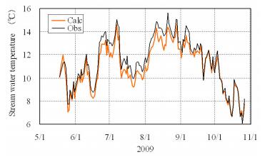 Figure 14. Comparison between the daily mean calculated and observed stream water temperatures at site P3 in May–October 2009.
Figure 15 shows analytical results of the sensitivity for the stream temperature simulations at site P3 on the fine days during the foliation (24–25 June). The constant shading factors of 0.1 and 0.6 were applied to the simulations, corresponding to the shaded condition at site P1 (Figure 8 and Figure 11) and the pre-foliation or nearly the de-foliation at site P3 (Figure 9 and Figure 11), respectively. Stream water temperature at the shading factors of 0.1 and 0.6 was overestimated by more than 5 ℃ on the daytime. This indicates that the shading factor strongly influences the stream water temperature on the daytime. Actually, the shading factor calculated for the simulated period of 24–25 June hardly changes along the stream channels with the average of 0.84 (Figure 11). Hence, the constant shading factor of 0.84 may give a reasonable simulated result as well.
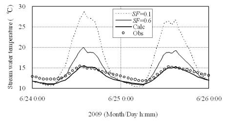 Figure 15. Sensitivity analysis for stream water temperature time series at site P3 by changing the shading factor (SF). The constant shading factors of SF = 0.1 (dashed line) and SF = 0.6 (thin solid line) were applied. The labels, "Calc" (bold solid line) and "Obs" (circle) indicate the calculated stream temperature by the variable shading factors and the observed stream temperature, respectively.
In this study, the stream heat budget was calculated to determine environmental factors controlling the stream water temperature in the forest catchment. In order to quantify the incoming and outgoing radiations for the forest stream, the hemispherical photographs were taken and the shading factors were calculated at several sites along the stream channels in the pre-foliation, foliation and defoliation periods of May to October. The shading factors exhibited both seasonal and spatial changes impressing variabilities of time scale and space on the shortwave and longwave radiations. The relatively small wind speed was observed above the stream in forest, compared with that in the open field, which produced the turbulent heat fluxes one third as large as in the open field. The wind direction was then distributed roughly along the channels. Thus, the stream channel could be a main wind pathway, and the wind above stream surface possibly follows the log law of wind velocity. The calculation of the heat budget revealed that the shortwave and longwave radiations and the advective heat flux from the upstream provide the major contribution. The streambed heat conduction exhibited the secondary contribution.
The stream water temperature was simulated by using the calculated stream heat budget. As a result, the simulations were consistent at RMSE = 0.771 ℃ and NASH = 0.888. Hence, the quantification of the shade at stream surface and the estimate of the heat budget are judged to be reasonable. However, the RMSE value at 0.771 ℃ is larger than the accuracy, 0.2 ℃, of temperature loggers. This is probably due to the underestimate of the heat exchange Hsurf at water surface in Eq 4. In this study, topographic effects around the stream channel on Hsurf are neglected, which tends to underestimate the incoming longwave radiation and evaporative and sensible heat fluxes at stream surface. Also, the wind speed above the forest stream is at any time less than 1 m s-1, giving small He and Hs values in Eqs 10 and 11. Hence, the application of the bulk method may have a problem for the forest stream.
The sensitivity analysis revealed that the shading factor highly control the stream water temperature, especially on the daytime. It is necessary (1) to take hemispherical photographs at different heights, in order to more properly estimate the shade by the stream bank, (2) to more properly estimate the shade by direct measurement of the shortwave and longwave radiations above the stream, because of the incomplete opacity and body temperature of leaves, (3) to more accurately calculate the advective heat flux during rainfall events, and (4) to simulate stream water temperature by considering the topographic effect around the stream channel.
I am greatly indebted to Mr. R. Kaminaga and Mr. M. Hayashi, graduate students of Laboratory of Physical Hydrology, Division of Natural History Sciences, Graduate School of Science, Hokkaido University, and Mr. H. Kan-no and Mr. J. Nagase and the Kitami-city for their welcome support during the field observations, and to Mr. H. Kitano, the principal of the Mizuho elementary-junior high school, for the kind permission of setting the weather station. I express my thanks to the Abashiri District Public Works Management Office for the welcome data supply of rainfalls.
All authors declare no conflicts of interest in this paper.
| [1] |
Webb BW, Hannah DM, Moore RD, et al. (2008) Recent advances in stream and river temperature research. Hydrol Proc 22: 902–918. doi: 10.1002/hyp.6994

|
| [2] |
Webb BW, Zhang Y (1997) Spatial and seasonal variability in the components of the river heat budget. Hydrol Proc 11: 79–101. doi: 10.1002/(SICI)1099-1085(199701)11:1<79::AID-HYP404>3.0.CO;2-N
|
| [3] |
Webb BW, Zhang Y (1999) Water temperatures and heat budgets in Dorset chalk water courses. Hydrol Proc 13: 309–321. doi: 10.1002/(SICI)1099-1085(19990228)13:3<309::AID-HYP740>3.0.CO;2-7
|
| [4] |
Moore RD, Sutherland P, Gomi T, et al. (2005) Thermal regime of a headwater stream within a clear-cut, coastal British Columbia, Canada. Hydrol Proc 19: 2591–2608. doi: 10.1002/hyp.5733
|
| [5] |
Hannah DM, Malcolm IA, Soulsby C, et al. (2008) A comparison of forest and moorland stream microclimate, heat exchanges and thermal dynamics. Hydrol Proc 22: 919–940. doi: 10.1002/hyp.7003
|
| [6] | Benyahya L, Caissie D, El-Jabi N, et al. (2010) Comparison of microclimate vs. remote meteorological data and results applied to a water temperature model (Miramichi River, Canada). Jour Hydrol 380: 247–259. |
| [7] | Nakamura F, Dokai T (1989) Estimation of the effect of riparian forest on stream temperature based on heat budget. Jour Jap Forestry Soc 71: 387–394. |
| [8] |
Sugimoto S, Nakamura F, Ito A (1997) Heat budget and statistical analysis of the relationship between stream temperature and riparian forest in the Toikanbetsu River basin, Northern Japan. Jour Forest Res 2: 103–107. doi: 10.1007/BF02348477
|
| [9] | Dugdale SJ, Malcolm IA, Kantola K, et al. (2018) Stream temperature under contrasting riparian forest cover: Understanding thermal dynamics and heat exchange processes. Sci Total Environ 610–611: 1375–1389. |
| [10] | Geological Survey of Hokkaido. (2004) The geology in Abashiri, Hokkaido, Japan. II The north and middle Abashiri (in Japanese). |
| [11] |
Baxter C, Hauer FR, Woessner WW (2003) Measuring groundwater-stream water exchange: new techniques for installing minipiezometers and estimating hydraulic conductivity. Trans Amer Fish Soc 132: 493–502. doi: 10.1577/1548-8659(2003)132<0493:MGWENT>2.0.CO;2
|
| [12] | Franzer GW, Canham CD, Lertzman KP (1999) Gap Light Analyzer (GLA), version 2.0: Imaging software to extract canopy structure and gap light transmission indices from true-colour fisheye photographs. User's Manual and Program Documentation. Simon Fraser University, Burnaby, B.C. and the Institute of Ecosystem Studies, Millbrook, NY. |
| [13] |
Kell GS (1975) Density, thermal expansivity, and compressibility of liquid water from 0 ℃ to 150 ℃: Correlations and tables for atmospheric pressure and saturation reviewed and expressed on 1968 temperature scale. Jour Chem Eng Data 20: 97–105. doi: 10.1021/je60064a005
|
| [14] | Chikita KA, Kaminaga R, Kudo I, et al. (2009) Parameters determining water temperature of a glacial stream: The Phelan Creek and the Gulkana Glacier, Alaska. River Res Applic 26: 995–1004. |
| [15] |
McMahon A, Moore RD (2017) Influence of turbidity and aeration on the albedo of mountain streams. Hydrol Proc 31: 4477–4491. doi: 10.1002/hyp.11370
|
| [16] |
Caissie D, Satish MG, El-Jabi N (2007) Predicting water temperatures using a deterministic model: Application on Miramichi River catchments (New Brunswick, Canada). Jour Hydrol 336: 303–315. doi: 10.1016/j.jhydrol.2007.01.008
|
| [17] | Morin G, Couillard D (1990) Predicting river temperatures with a hydrological model. Encyclopedia of Fluid Mechanic, Surface and Groundwater Flow Phenomena, 10, Houston, TX: Gulf Publishing Company, 171–209. |
| [18] | Maidment DR (1992) Handbook of Hydrology. New York: McGraw-Hill. |
| [19] | Theurer FD, Voos KA, Miller WJ (1984) Instream water temperature model. US Fish and Wildlife Service Instream Flow Information Paper 16, 200. |
| [20] | Kondo J (1994) Meteorology in aquatic environments. Tokyo, Japan: Asakura Publishing Ltd., 350. |
| 1. | Sooyoun Nam, Su-Jin Jang, Kun-Woo Chun, Jae Uk Lee, Suk Woo Kim, Seasonal water temperature variations in response to air temperature and precipitation in a forested headwater stream and an urban river: a case study from the Bukhan River basin, South Korea, 2021, 2158-0103, 1, 10.1080/21580103.2021.1882589 | |
| 2. | Iman Maghami, Victor A. L. Sobral, Mohamed M. Morsy, John C. Lach, Jonathan L. Goodall, Exploring the complementary relationship between solar and hydro energy harvesting for self-powered water monitoring in low-light conditions, 2021, 140, 13648152, 105032, 10.1016/j.envsoft.2021.105032 | |
| 3. | Nicole Durfee, Carlos G. Ochoa, Gerrad Jones, Stream Temperature and Environment Relationships in a Semiarid Riparian Corridor, 2021, 10, 2073-445X, 519, 10.3390/land10050519 |

Kazuhisa A. Chikita. Environmental factors controlling stream water temperature in a forest catchment[J]. AIMS Geosciences, 2018, 4(4): 192-214. doi: 10.3934/geosci.2018.4.192

| Site | SR | ILR | OLR | EH | SH | |||||
| P7 | 27.9 | (28.4%) | 67.7 | (68.9%) | -73.6 | (-100%) | 0.9 | (0.9%) | 1.8 | (1.8%) |
| P6 | 32.3 | (28.4%) | 79.2 | (69.6%) | -87.0 | (-100%) | 0.7 | (0.6%) | 1.6 | (1.4%) |
| P5 | 28.5 | (27.9%) | 71.9 | (70.3%) | -79.7 | (-100%) | 0.4 | (0.4%) | 1.5 | (1.4%) |
| P3 | 29.3 | (28.1%) | 73.4 | (70.3%) | -81.1 | (-100%) | 0.3 | (0.3%) | 1.4 | (1.3%) |
| P1 | 127 | (28.8%) | 311 | (70.3%) | -344 | (-99.6%) | -1.5 | (-0.4%) | 4.4 | (1.0%) |
DownLoad: CSV| Site | SR | ILR | OLR | EH | SH | |||||
| P7 | 27.9 | (28.4%) | 67.7 | (68.9%) | -73.6 | (-100%) | 0.9 | (0.9%) | 1.8 | (1.8%) |
| P6 | 32.3 | (28.4%) | 79.2 | (69.6%) | -87.0 | (-100%) | 0.7 | (0.6%) | 1.6 | (1.4%) |
| P5 | 28.5 | (27.9%) | 71.9 | (70.3%) | -79.7 | (-100%) | 0.4 | (0.4%) | 1.5 | (1.4%) |
| P3 | 29.3 | (28.1%) | 73.4 | (70.3%) | -81.1 | (-100%) | 0.3 | (0.3%) | 1.4 | (1.3%) |
| P1 | 127 | (28.8%) | 311 | (70.3%) | -344 | (-99.6%) | -1.5 | (-0.4%) | 4.4 | (1.0%) |


