Research article

Influence of Climate Factors on Rice Yields in Cambodia

  • Received: 19 March 2017 Accepted: 15 December 2017 Published: 22 December 2017
  • Temperature and precipitation have been known as the key determinant factors to affect rice production in climate change. In this study, the relationship between climate variables and rice yields during 1993–2012 in Cambodia was analyzed and evaluated. The Ordinary Least Squares analysis was applied to examine the relationship of three climate variables (TCV) including maximum temperature, minimum temperature and rainfall against seasonal rice yields. By this period, a remarkable increasing trend of annual temperature was observed whilst rainfall was not significantly changed. The TCV explains approximately 63% and 56% of the variability of rice yields in wet and dry seasons, respectively. It is found that in Cambodia, non-climate factors such as fertilizers, water, cultivars, and soil fertility cause 40% variation to rice yields, whereas the remaining 60% can be influenced by climate variability. The levels of temperature difference (LTD) between maximum and minimum temperatures of the wet season (WS) and dry season (DS) were 7.0 and 8.6 oC, respectively. The lower value of LTD may cause the reduction of rice in WS (2.2 tons/ha) as compared to that of DS (3.0 tons/ha). Rice yield has increased 50.5% and 33.8% in DS and WS, respectively, may due to the improvement of rice cultivation practices in Cambodia such as the better use of fertilizers, pest and weed control, and irrigation, and more effective rice cultivated protocol, as the increased trend of temperature may detrimentally affect rice yield. The breeding of heat and drought tolerance rice varieties and development of irrigation system are effective to reduce the negative influence from climate change to rice production in Cambodia.

    Citation: Dek Vimean Pheakdey, Tran Dang Xuan, Tran Dang Khanh. Influence of Climate Factors on Rice Yields in Cambodia[J]. AIMS Geosciences, 2017, 3(4): 561-575. doi: 10.3934/geosci.2017.4.561

    Related Papers:

    [1] Lunyi Liu, Qunying Wu . Complete integral convergence for weighted sums of negatively dependent random variables under sub-linear expectations. AIMS Mathematics, 2023, 8(9): 22319-22337. doi: 10.3934/math.20231138
    [2] Mingzhou Xu, Kun Cheng, Wangke Yu . Complete convergence for weighted sums of negatively dependent random variables under sub-linear expectations. AIMS Mathematics, 2022, 7(11): 19998-20019. doi: 10.3934/math.20221094
    [3] Mingzhou Xu . Complete convergence and complete moment convergence for maximal weighted sums of extended negatively dependent random variables under sub-linear expectations. AIMS Mathematics, 2023, 8(8): 19442-19460. doi: 10.3934/math.2023992
    [4] Shuyan Li, Qunying Wu . Complete integration convergence for arrays of rowwise extended negatively dependent random variables under the sub-linear expectations. AIMS Mathematics, 2021, 6(11): 12166-12181. doi: 10.3934/math.2021706
    [5] Mingzhou Xu . On the complete moment convergence of moving average processes generated by negatively dependent random variables under sub-linear expectations. AIMS Mathematics, 2024, 9(2): 3369-3385. doi: 10.3934/math.2024165
    [6] He Dong, Xili Tan, Yong Zhang . Complete convergence and complete integration convergence for weighted sums of arrays of rowwise $ m $-END under sub-linear expectations space. AIMS Mathematics, 2023, 8(3): 6705-6724. doi: 10.3934/math.2023340
    [7] Chengcheng Jia, Qunying Wu . Complete convergence and complete integral convergence for weighted sums of widely acceptable random variables under the sub-linear expectations. AIMS Mathematics, 2022, 7(5): 8430-8448. doi: 10.3934/math.2022470
    [8] Mingzhou Xu . Complete convergence of moving average processes produced by negatively dependent random variables under sub-linear expectations. AIMS Mathematics, 2023, 8(7): 17067-17080. doi: 10.3934/math.2023871
    [9] Xiaocong Chen, Qunying Wu . Complete convergence and complete integral convergence of partial sums for moving average process under sub-linear expectations. AIMS Mathematics, 2022, 7(6): 9694-9715. doi: 10.3934/math.2022540
    [10] Haiwu Huang, Yuan Yuan, Hongguo Zeng . An extension on the rate of complete moment convergence for weighted sums of weakly dependent random variables. AIMS Mathematics, 2023, 8(1): 622-632. doi: 10.3934/math.2023029
  • Temperature and precipitation have been known as the key determinant factors to affect rice production in climate change. In this study, the relationship between climate variables and rice yields during 1993–2012 in Cambodia was analyzed and evaluated. The Ordinary Least Squares analysis was applied to examine the relationship of three climate variables (TCV) including maximum temperature, minimum temperature and rainfall against seasonal rice yields. By this period, a remarkable increasing trend of annual temperature was observed whilst rainfall was not significantly changed. The TCV explains approximately 63% and 56% of the variability of rice yields in wet and dry seasons, respectively. It is found that in Cambodia, non-climate factors such as fertilizers, water, cultivars, and soil fertility cause 40% variation to rice yields, whereas the remaining 60% can be influenced by climate variability. The levels of temperature difference (LTD) between maximum and minimum temperatures of the wet season (WS) and dry season (DS) were 7.0 and 8.6 oC, respectively. The lower value of LTD may cause the reduction of rice in WS (2.2 tons/ha) as compared to that of DS (3.0 tons/ha). Rice yield has increased 50.5% and 33.8% in DS and WS, respectively, may due to the improvement of rice cultivation practices in Cambodia such as the better use of fertilizers, pest and weed control, and irrigation, and more effective rice cultivated protocol, as the increased trend of temperature may detrimentally affect rice yield. The breeding of heat and drought tolerance rice varieties and development of irrigation system are effective to reduce the negative influence from climate change to rice production in Cambodia.


    Peng [1,2] introduced seminal concepts of the sub-linear expectations space to study the uncertainty in probability. The works of Peng [1,2] stimulate many scholars to investigate the results under sub-linear expectations space, extending those in classic probability space. Zhang [3,4] got exponential inequalities and Rosenthal's inequality under sub-linear expectations. For more limit theorems under sub-linear expectations, the readers could refer to Zhang [5], Xu and Zhang [6,7], Wu and Jiang [8], Zhang and Lin [9], Zhong and Wu [10], Chen [11], Chen and Wu [12], Zhang [13], Hu et al. [14], Gao and Xu [15], Kuczmaszewska [16], Xu and Cheng [17,18,19], Xu et al. [20] and references therein.

    In probability space, Shen et al. [21] obtained equivalent conditions of complete convergence and complete moment convergence for extended negatively dependent random variables. For references on complete moment convergence and complete convergence in probability space, the reader could refer to Hsu and Robbins [22], Chow [23], Ko [24], Meng et al. [25], Hosseini and Nezakati [26], Meng et al. [27] and refercences therein. Inspired by the work of Shen et al. [21], we try to investigate complete convergence and complete moment convergence for negatively dependent (ND) random variables under sub-linear expectations, and the Marcinkiewicz-Zygmund type result for ND random variables under sub-linear expectations, which complements the relevant results in Shen et al. [21].

    Recently, Srivastava et al. [28] introduced and studied comcept of statistical probability convergence. Srivastava et al. [29] investigated the relevant results of statistical probability convergence via deferred Nörlund summability mean. For more recent works, the interested reader could refer to Srivastava et al. [30,31,32], Paikary et al. [33] and references therein. We conjecture the relevant notions and results of statistical probability convergence could be extended to that under sub-linear expectation.

    We organize the remainders of this article as follows. We cite relevant basic notions, concepts and properties, and present relevant lemmas under sub-linear expectations in Section 2. In Section 3, we give our main results, Theorems 3.1 and 3.2, the proofs of which are given in Section 4.

    In this article, we use notions as in the works by Peng [2], Zhang [4]. Suppose that (Ω,F) is a given measurable space. Assume that H is a collection of all random variables on (Ω,F) satisfying φ(X1,,Xn)H for X1,,XnH, and each φCl,Lip(Rn), where Cl,Lip(Rn) represents the space of φ fulfilling

    |φ(x)φ(y)|C(1+|x|m+|y|m)(|xy|),x,yRn

    for some C>0, mN relying on φ.

    Definition 2.1. A sub-linear expectation E on H is a functional E:HˉR:=[,] fulfilling the following: for every X,YH,

    (a) XY yields E[X]E[Y];

    (b) E[c]=c, cR;

    (c) E[λX]=λE[X], λ0;

    (d) E[X+Y]E[X]+E[Y] whenever E[X]+E[Y] is not of the form or +.

    We name a set function V:F[0,1] a capacity if

    (a)V()=0, V(Ω)=1;

    (b)V(A)V(B), AB, A,BF.

    Moreover, if V is continuous, then V obey

    (c) AnA concludes V(An)V(A);

    (d) AnA concludes V(An)V(A).

    V is named to be sub-additive when V(A+B)V(A)+V(B), A,BF.

    Under the sub-linear expectation space (Ω,H,E), set V(A):=inf{E[ξ]:IAξ,ξH}, AF (cf. Zhang [3,4,9,13], Chen and Wu [12], Xu et al. [20]). V is a sub-additive capacity. Set

    V(A)=inf{n=1V(An):An=1An},AF.

    By Definition 4.2 and Lemma 4.3 of Zhang [34], if E=E is linear expectation, V coincide with the probability measure introduced by the linear expectation E. As in Zhang [3], V is countably sub-additive, V(A)V(A). Hence, in Theorem 3.1, Corollary 3.1, V could be replaced by V, implying that the results here could be considered as natural extensions of the corresponding ones in classic probability space. Write

    CV(X):=0V(X>x)dx+0(V(X>x)1)dx.

    Assume X=(X1,,Xm), XiH and Y=(Y1,,Yn), YiH are two random vectors on (Ω,H,E). Y is called to be negatively dependent to X, if for ψ1 on Cl,Lip(Rm), ψ2 on Cl,Lip(Rn), we have E[ψ1(X)ψ2(Y)]E[ψ1(X)]E[ψ2(Y)] whenever ψ1(X)0, E[ψ2(Y)]0, E[|ψ1(X)ψ2(Y)|]<, E[|ψ1(X)|]<, E[|ψ2(Y)|]<, and either ψ1 and ψ2 are coordinatewise nondecreasing or ψ1 and ψ2 are coordinatewise nonincreasing (cf. Definition 2.3 of Zhang [3], Definition 1.5 of Zhang [4]).

    {Xn}n=1 is called to be negatively dependent, if Xn+1 is negatively dependent to (X1,,Xn) for each n1. The existence of negatively dependent random variables {Xn}n=1 under sub-linear expectations could be yielded by Example 1.6 of Zhang [4] and Kolmogorov's existence theorem in classic probabililty space. We below give an concrete example.

    Example 2.1. Let P={Q1,Q2} be a family of probability measures on (Ω,F). Suppose that {Xn}n=1 are independent, identically distributed under each Qi, i=1,2 with Q1(X1=1)=Q1(X1=1)=1/2, Q2(X1=1)=1. Define E[ξ]=supQPEQ[ξ], for each random variable ξ. Here E[] is a sub-linear expectation. By the discussion of Example 1.6 of Zhang [4], we see that {Xn}n=1 are negatively dependent random variables under E.

    Assume that X1 and X2 are two n-dimensional random vectors in sub-linear expectation spaces (Ω1,H1,E1) and (Ω2,H2,E2) repectively. They are named identically distributed if for every ψCl,Lip(Rn),

    E1[ψ(X1)]=E2[ψ(X2)]. 

    {Xn}n=1 is called to be identically distributed if for every i1, Xi and X1 are identically distributed.

    In this article we assume that E is countably sub-additive, i.e., E(X)n=1E(Xn) could be implied by Xn=1Xn, X,XnH, and X0, Xn0, n=1,2,. Write Sn=ni=1Xi, n1. Let C denote a positive constant which may vary in different occasions. I(A) or IA represent the indicator function of A. The notion axbx means that there exist two positive constants C1, C2 such that C1|bx||ax|C2|bx|.

    As in Zhang [4], by definition, if X1,X2,,Xn are negatively dependent random variables and f1, f2,,fn are all non increasing (or non decreasing) functions, then f1(X1), f2(X2),,fn(Xn) are still negatively dependent random variables.

    We cite the useful inequalities under sub-linear expectations.

    Lemma 2.1. (See Lemma 4.5 (III) of Zhang [3]) If E is countably sub-additive under (Ω,H,E), then for XH,

    E|X|CV(|X|).

    Lemma 2.2. (See Lemmas 2.3, 2.4 of Xu et al. [20] and Theorem 2.1 of Zhang [4]) Assume that p1 and {Xn;n1} is a sequence of negatively dependent random varables under (Ω,H,E). Then there exists a positive constant C=C(p) relying on p such that

    E[|nj=1Xj|p]C{ni=1E|Xi|p+(ni=1[|E(Xi)|+|E(Xi)|])p},1p2, (2.1)
    E[max1in|ij=1Xj|p]C(logn)p{ni=1E|Xi|p+(ni=1[|E(Xi)|+|E(Xi)|])p},1p2, (2.2)
    E[max1in|ij=1Xi|p]C{ni=1E|Xi|p+(ni=1EX2i)p/2+(ni=1[|E(Xi)|+|E(Xi)|])p},p2. (2.3)

    Lemma 2.3. Assume that XH, α>0, γ>0, CV(|X|α)<. Then there exists a positive constant C relying on α,γ such that

    0V{|X|>γy}yα1dyCCV(|X|α)<.

    Proof. By the method of substitution of definite integral, letting γy=z1/α, we get

    0V{|X|>γy}yα1dy0V{|X|α>z}(z1/α/γ)α1z1/α1/γdzCCV(|X|α)<.

    Lemma 2.4. Let Yn,ZnH. Then for any q>1, ε>0 and a>0,

    E(max1jn|ji=1(Yi+Zi)|εa)+(1εq+1q1)1aq1E(max1jn|ji=1Yi|q)+E(max1jn|ji=1Zi|). (2.4)

    Proof. By Markov' inequality under sub-linear expectations, Lemma 2.1, and the similar proof of Lemma 2.4 of Sung [35], we could finish the proof. Hence, the proof is omitted here.

    Our main results are below.

    Theorem 3.1. Suppose α>12 and αp>1. Assume that {Xn,n1} is a sequence of negatively dependent random variables, and for each n1, Xn is identically distributed as X under sub-linear expectation space (Ω,H,E). Moreover, assume E(X)=E(X)=0 if p1. Suppose CV(|X|p)<. Then for all ε>0,

    n=1nαp2V{max1jn|ji=1Xi|>εnα}<. (3.1)

    Remark 3.1. By Example 2.1, the assumption E(X)=E(X)=0 if p1 in Theorem 3.1 can not be weakened to E(X)=0 if p1. In fact, in the case of Example 2.1, if 12<α1, αp>1, then for any 0<ε<1,

    n=1nαp2V{max1jn|ji=1Xi|>εnα}n=1nαp2V{max1jn|ji=1Xi|n}=n=1nαp2=+,

    which implies that Theorems 3.1, 3.2, Corollary 3.1 do not hold. However, by Example 1.6 of Zhang [4], the assumptions of Theorem 3.3, Corollary 3.2 hold for random variables in Example 2.1, hence Theorem 3.3, Corollary 3.2 are valid in this example.

    By Theorem 3.1, we could get the Marcinkiewicz-Zygmund strong law of large numbers for negatively dependent random variables under sub-linear expectations below.

    Corollary 3.1. Let α>12 and αp>1. Assume that under sub-linear expectation space (Ω,H,E), {Xn} is a sequence of negatively dependent random variables and for each n, Xn is identically distributed as X. Moreover, assume E(X)=E(X)=0 if p1. Assume that V induced by E is countably sub-additive. Suppose CV{|X|p}<. Then

    V(lim supn1nα|ni=1Xi|>0)=0. (3.2)

    Theorem 3.2. If the assumptions of Theorem 3.1 hold for p1 and CV{|X|plogθ|X|}< for some θ>max{αp1α12,p}, then for any ε>0,

    n=1nαp2αE(max1jn|ji=1Xi|εnα)+<. (3.3)

    By the similar proof of Theorem 3.1, with Theorem 2.1 (b) for negative dependent random variables of Zhang [4] (cf. the proof of Theorem 2.1 (c) there) in place of Lemma 2.2 here, we could obtain the following result.

    Theorem 3.3. Suppose α>12, p1, and αp>1. Assume that Xk is negatively dependent to (Xk+1,,Xn), for each k=1,,n, n1. Suppose for each n, Xn is identically distributed as X under sub-linear expectation space (Ω,H,E). Suppose CV(|X|p)<. Then for all ε>0,

    n=1nαp2V{max1jnji=1[XiE(Xi)]>εnα}<,
    n=1nαp2V{max1jnji=1[XiE(Xi)]>εnα}<.

    By the similar proof of Corollary 3.1, with Theorem 3.3 in place of Theorem 3.1, we get the following result.

    Corollary 3.2. Let α>12, p1, and αp>1. Assume that Xk is negatively dependent to (Xk+1,,Xn), for each k=1,,n, n1. Suppose for each n, Xn is identically distributed as X under sub-linear expectation space (Ω,H,E). Assume that V induced by E is countably sub-additive. Suppose CV{|X|p}<. Then

    V({lim supn1nαni=1[XiE(Xi)]>0}{lim supn1nαni=1[XiE(Xi)]>0})=0.

    By the similar proof of Theorem 3.1 and Corollary 3.1, and adapting the proof of (4.10), we could obtain the following result.

    Corollary 3.3. Suppose α>1 and p1. Assume that {Xn,n1} is a sequence of negatively dependent random variables, and for each n1, Xn is identically distributed as X under sub-linear expectation space (Ω,H,E). Suppose CV(|X|p)<. Then for all ε>0,

    n=1nαp2V{max1jnji=1[XiE(Xi)]>εnα}<,
    n=1nαp2V{max1jnji=1[XiE(Xi)]>εnα}<.

    Moreover assume that V induced by E is countably sub-additive. Then

    V({lim supn1nαni=1[XiE(Xi)]>0}{lim supn1nαni=1[XiE(Xi)]>0})=0.

    By the discussion below Definition 4.1 of Zhang [34], and Corollary 3.2, we conjecture the following.

    Conjecture 3.1. Suppose 12<α1 and αp>1. Assume that {Xn,n1} is a sequence of negatively dependent random variables, and for each n1, Xn is identically distributed as X under sub-linear expectation space (Ω,H,E). Assume that V induced by E is continuous. Suppose CV{|X|p}<. Then

    V({lim supn1nαni=1[XiE(Xi)]>0}{lim supn1nαni=1[XiE(Xi)]>0})=0.

    Proof of Theorem 3.1. We investigate the following cases.

    Case 1. 0<p<1.

    For fixed n1, for 1in, write

    Yni=nαI{Xi<nα}+XiI{|Xi|nα}+nαI{Xi>nα},
    Zni=(Xinα)I{Xi>nα}+(Xi+nα)I{Xi<nα},
    Yn=nαI{X<nα}+XI{|X|nα}+nαI{X>nα},
    Zn=XYn.

    Observing that Xi=Yni+Zni, we see that for all ε>0,

    n=1nαp2V{max1jn|ji=1Xi|>εnα}n=1nαp2V{max1jn|ji=1Yni|>εnα/2}+n=1nαp2V{max1jn|ji=1Zni|>εnα/2}=:I1+I2. (4.1)

    By Markov's inequality under sub-linear expectations, Cr inequality, and Lemmas 2.1, 2.3, we conclude that

    I1Cn=1nαp2αni=1E|Yni|=Cn=1nαp1αE|Yn|Cn=1nαp1αCV(|Yn|)Cn=1nαp1αnα0V{|Yn|>x}dx=Cn=1nαp1αnk=1kα(k1)αV{|X|>x}dx=Ck=1kα(k1)αV{|X|>x}dxn=knαp1α=Ck=1kα1V{|X|>(k1)α}kαpαCk=1kαp1V{|X|>kα}+CC0xαp1V{|X|>xα}dx+CCCV{|X|p}+C<, (4.2)

    and

    I2Cn=1nαp2αp/2ni=1E|Zni|p/2Cn=1nαp/21E|Zn|p/2Cn=1nαp/21CV{|Zn|p/2}Cn=1nαp/21CV{|X|p/2I{|X|>nα}}Cn=1nαp/21[nα0V{|X|>nα}sp/21ds+nαV{|X|>s}sp/21ds]Cn=1nαp1V{|X|>nα}+Cn=1nαp/21k=n(k+1)αkαV{|X|>s}sp/21dsCCV{|X|p}+Ck=1(k+1)αkαV{|X|>s}sp/21dskn=1nαp/21CCV{|X|p}+Ck=1V{|X|>kα}kαp1CCV{|X|p}+CCV{|X|p}<. (4.3)

    Therefore, by (4.1)–(4.3), we deduce that (3.1) holds.

    Case 2. p1.

    Observing that αp>1, we choose a suitable q such that 1αp<q<1. For fixed n1, for 1in, write

    X(1)ni=nαqI{Xi<nαq}+XiI{|Xi|nαq}+nαqI(Xi>nαq),
    X(2)ni=(Xinαq)I{Xi>nαq},X(3)ni=(Xi+nαq)I{Xi<nαq},

    and X(1)n, X(2)n, X(3)n is defined as X(1)ni, X(2)ni, X(3)ni only with X in place of Xi above. Observing that ji=1Xi=ji=1X(1)ni+ji=1X(2)ni+ji=1X(3)ni, for 1jn, we see that for all ε>0,

    n=1nαp2V{max1jn|ji=1Xi|>εnα}n=1nαp2V{max1jn|ji=1X(1)ni|>εnα/3}+n=1nαp2V{max1jn|ji=1X(2)ni|>εnα/3}+n=1nαp2V{max1jn|ji=1X(3)ni|>εnα/3}=:II1+II2+II3. (4.4)

    Therefore, to establish (3.1), it is enough to prove that II1<, II2<, II3<.

    For II1, we first establish that

    nαmax1jn|ji=1EX(1)ni|0, as n. (4.5)

    By E(X)=0, Markov's inequality under sub-linear expectations, Lemma 2.1, we conclude that

    nαmax1jn|ji=1EX(1)ni|nαni=1|E(X(1)n)|n1α|E(X(1)n)E(X)|n1αE|X(1)nX|n1αCV(|X(1)nX|)Cn1α[0V{|X|I{|X|>nαq}>x}dx]Cn1α[nαq0V{|X|>nαq}dx+nαqV{|X|>y}dy]Cn1α+αqV{|X|>nαq}+Cn1αnαqV{|X|>y}yp1nαq(p1)dyCn1α+αqE|X|pnαqp+Cn1α+αqαqpCV{|X|p}Cn1αqpα+αqCV{|X|p},

    which results in (4.5) by CV{|X|p}< and 1/(αp)<q<1. Thus, from (4.5), it follows that

    II1Cn=1nαp2V{max1jn|ji=1(X(1)niEX(1)ni)|>εnα6}. (4.6)

    For fixed n1, we note that {X(1)niEX(1)ni,1in} are negatively dependent random variables. By (4.6), Markov's inequality under sub-linear expectations, and Lemma 2.2, we see that for any β2,

    II1Cn=1nαp2αβE(max1jn|ji=1(X(1)niEX(1)ni)|β)Cn=1nαp2αβ[ni=1E|X(1)ni|β+(ni=1E|X(1)ni|2)β/2+(ni=1[|EX(1)ni|+|E(X(1)ni)|])β]=:II11+II12+II13. (4.7)

    Taking β>max{αp1α1/2,2,p,αp1αqpαq+α1}, we obtain

    αpαβ+αqβαpq1=α(pβ)(1q)1<1,
    αp2αβ+β/2<1,

    and

    αp2αβ+βαq(p1)β<1.

    By Cr inequality, Markov's inequality under sub-linear expectations, Lemma 2.1, we see that

    II11Cn=1nαp2αβni=1E|X(1)ni|βCn=1nαp1αβE|X(1)n|βCn=1nαp1αβCV{|X(1)n|β}=Cn=1nαp1αβnαqβ0V{|X|β>x}dxCn=1nαp1αβnαq0V{|X|>x}xβ1dxCn=1nαp1αβnαq0V{|X|>x}xp1nαq(βp)dxCn=1nαp1αβ+αqβαqpCV{|X|p}<, (4.8)
    II12Cn=1nαp2αβ(ni=1E|X(1)n|2)β/2Cn=1nαp2αβ+β/2(CV{|X(1)n|2})β/2Cn=1nαp2αβ+β/2(nαq0V{|X|>x}xdx)β/2{Cn=1nαp2αβ+β/2(CV{|X|2})β/2, if p2;Cn=1nαp2αβ+β/2(nαq0V{|X|>x}xp1nαq(2p)dx)β/2, if 1p<2,{Cn=1nαp2αβ+β/2(CV{|X|2})β/2<, if p2;Cn=1n(αp1)(1β/2)1(CV(|X|p))β/2<, if 1p<2, (4.9)

    and

    II13Cn=1nαp2αβ(ni=1[|EX(1)n|+|E(X(1)n)|])βCn=1nαp2αβ+β(E|X(1)nX|)βCn=1nαp2αβ+β(E|X|p)βnαq(p1)βCn=1nαp2αβ+βαq(p1)β(CV(|X|p))β<. (4.10)

    Therefore, combining (4.7)–(4.10) results in II1<.

    Next, we will establish that II2<. Let gμ(x) be a non-increasing Lipschitz function such that I{xμ}gμ(x)I{x1}, μ(0,1). Obviously, I{x>μ}>1gμ(x)>I{x>1}. For fixed n1, for 1in, write

    X(4)ni=(Xinαq)I(nαq<Xinα+nαq)+nαI(Xi>nα+nαq),

    and

    X(4)n=(Xnαq)I(nαq<Xnα+nαq)+nαI(X>nα+nαq).

    We see that

    (max1jn|ij=1X(2)ni|>εnα3)(max1in|Xi|>nα)(max1jn|ij=1X(4)ni|>εnα3),

    which results in

    II2n=1nαp2ni=1V{|Xi|>nα}+n=1nαp2V{max1jn|ij=1X(4)ni|>εnα3}=:II21+II22. (4.11)

    By CV{|X|p}<, we conclude that

    II21Cn=1nαp2ni=1E[1gμ(|Xi|)]=Cn=1nαp1E[1gμ(|X|)]Cn=1nαp1V{|X|>μnα}C0xαp1V{|X|>μxα}dxCCV(|X|p)<. (4.12)

    Observing that 1αp<q<1, from the definition of X(2)ni, follows that

    nαmax1jn|ji=1EX(4)ni|Cn1αE|X(4)n|Cn1αCV(|X(4)n|)Cn1α[nαq0V{|X|I{|X|>nαq}>x}dx+nαqV{|X|>x}dx]Cn1α+αqE|X|pnαpq+Cn1αnαqV{|X|>x}xp1nαq(p1)dxCn1α+αqαpqCV{|X|p}0 as n. (4.13)

    By X(4)ni>0, (4.11)–(4.13), we see that

    II2Cn=1nαp2V{|ni=1[X(4)niEX(4)ni]|>εnα6}. (4.14)

    For fixed n1, we know that {X(4)niEX(4)ni,1in} are negatively dependent random variables under sub-linear expectations. By Markov's inequality under sub-linear expectations, Cr-inequality, Lemma 2.2, we obtain

    II2Cn=1nαp2αβE(|ni=1[X(4)niEX(4)ni]|β)Cn=1nαp2αβ[ni=1E|X(4)ni|β+(ni=1E(X(4)ni)2)β/2+(ni=1[|EX(4)ni|+|E(X(4)ni)|])β]=:II21+II22+II23. (4.15)

    By Cr inequality, Lemma 2.3, we have

    II21Cn=1nαp2αβni=1E|X(4)n|βCn=1nαp1αβCV{|X(4)n|β}Cn=1nαp1αβCV{|X|βI{nαq<Xnα+nαq}+nαqβI{X>nα+nαq}}Cn=1nαp1αβ2nα0V{|X|>x}xβ1dxCn=1nαp1αβnk=12kα2(k1)αV{|X|>x}xβ1dxCk=1V{|X|>2(k1)α}kαβ1n=knαp1αβCk=1V{|X|>2(k1)α}kαp1C0V{|X|>2xα}xαp1dxCCV{|X|p}<. (4.16)

    As in the proof of (4.9) and (4.16), we can deduce that II22<.

    By Lemma 2.1, we see that

    II23Cn=1nαp1αβnβ(E|X(4)n|)βCn=1nαp1αβ+β(E|X|pnαq(p1))βCn=1nαp1αβ+βαq(p1)(CV{|X|p})β<. (4.17)

    By (4.15)–(4.17), we deduce that II2<.

    As in the proof of II2<, we also can obtain II3<. Therefore, combining (4.5), II1<, II2<, and II3< results in (3.1). This finishes the proof.

    Proof of Corollary 3.1. By CV{|X|p}<, and Theorem 3.1, we deduce that for all ε>0,

    n=1nαp2V(max1jn|ji=1Xi|>εnα)<. (4.18)

    By (4.18), we conclude that for any ε>0,

    >n=1nαp2V(max1jn|ji=1Xi|>εnα)=k=02k+11n=2knαp2V(max1jn|ji=1Xi|>εnα){k=0(2k)αp22kV(max1j2k|ji=1Xi|>ε2(k+1)α), if αp2,k=0(2k+1)αp22kV(max1j2k|ji=1Xi|>ε2(k+1)α), if 1<αp<2,{k=0V(max1j2k|ji=1Xi|>ε2(k+1)α), if αp2,k=012V(max1j2k|ji=1Xi|>ε2(k+1)α), if 1<αp<2,

    which, combined with Borel-Cantell lemma under sub-linear expectations, yields that

    V(lim supnmax1j2k|ji=1Xi|2(k+1)α>0)=0. (4.19)

    For all positive integers n, a positive integer k satisfying 2k1n<2k, we see that

    nα|ni=1Xi|max2k1n2knα|ni=1Xi|22αmax1j2k|ji=1Xi|2(k+1)α,

    which yields (3.2). This completes the proof.

    Proof of Theorem 3.2. For fixed n1, for 1in, write

    Yni=nαI{Xi<nα}+XiI{|Xi|nα}+nαI{Xi>nα},
    Zni=XiYni=(Xinα)I{Xi>nα}+(Xi+nα)I{Xi<nα},

    and

    Yn=nαI{X<nα}+XI{|X|nα}+nαI{X>nα},
    Zn=XYn=(Xnα)I{X>nα}+(X+nα)I{X<nα}.

    From Lemma 2.4 follows that for any β>1,

    n=1nαp2αE(max1jn|ji=1Xi|εnα)+Cn=1nαp2αβE(max1jn|ji=1(YniEYni)|β)+n=1nαp2αE(max1jn|ji=1(ZniEZni)|)=:III1+III2. (4.20)

    Noticing that Zn(|X|nα)I(|X|>nα)|X|I(|X|>nα), by Lemma 2.3, we see that

    III2Cn=1nαp2αni=1E|Zni|Cn=1nαp1αE|Zn|Cn=1nαp1αCV{|Zn|}Cn=1nαp1αCV{|X|I(|X|>nα)}Cn=1nαp1α[nα0V{|X|>nα}dx+nαV{|X|>x}dx]Cn=1nαp1V{|X|>nα}+Cn=1nαp1αk=n(k+1)αkαV{|X|>x}dxCCV{|X|p}+Ck=1V{|X|>kα}kα1kn=1nαp1α{CCV{|X|p}+Ck=1V{|X|>kα}kα1log(k), if p=1,CCV{|X|p}+Ck=1V{|X|>kα}kαp1, if p>1,{CCV{|X|log|X|}<, if p=1,CCV{|X|p}<, if p>1. (4.21)

    Now, we will establish III1<. Observing that θ>p1, we can choose β=θ. We analysize the following two cases.

    Case 1. 1<θ2. From (2.2) of Lemma 2.2, Lemma 2.1, E(Y)=E(Y)=0, and Markov's inequality under sub-linear expectations follows that

    III1=Cn=1nαp2αθE(max1jn|ji=1(YniEYni)|θ)Cn=1nαp2αθlogθn[ni=1E|Yni|θ+(ni=1[|E(Yni)|+|E(Yni)|])θ]=Cn=1nαp2αθlogθn[ni=1E|Yn|θ+(ni=1[|E(Yn)|+|E(Yn)|])θ]Cn=1nαp1αθlogθnCV{|Yn|θ}+Cn=1nαp2αθ+θlogθn(E|YnX|)θCn=1nαp1αθlogθnnα0V{|X|>x}xθ1dx+Cn=1nαp2αθ+θlogθn(CV{|YnX|})θCn=1nαp1αθlogθnnk=1kα(k1)αV{|X|>x}xθ1dx+Cn=1nαp2αθ+θlogθn(CV{|X|I{|X|>nα}})θCk=1V{|X|>(k1)α}kαθ1n=knαp1αθ+Cn=1nαp2αθ+θlogθn(0V{|X|I{|X|>nα}>y}dy)θCk=1V{|X|>(k1)α}kαp1logθk+Cn=1nαp2αθ+θlogθn(nαE{|X|plogθ|X|}nαplogθn)θ+Cn=1nαp2αθ+θlogθn(nαV{|X|plogθ|X|>yplogθy}d(yplogθy)/(nα(p1)logθn))θC0V{|X|>xα}xαp1logθxdx+C(CV{|X|plogθ|X|})θ+Cn=1nαp2+θαpθlogθθ2n(CV{|X|plogθ|X|})θCCV{|X|plogθ|X|}+C(CV{|X|plogθ|X|})θ<. (4.22)

    Case 2. θ>2. Observe that θ>αp1α12, we conclude that αp2αθ+θ2<1. As in the proof of (4.22), by Lemma 2.2, and Cr inequality, we see that

    III1=Cn=1nαp2αθE(max1jn|ji=1(YniE(Yni))|θ)Cn=1nαp2αθ[ni=1E|Yni|θ+(ni=1E|Yni|2)θ/2+(ni=1[|E(Yni)|+|E(Yni)|])θ]=:III11+III12+III13. (4.23)

    By Lemma 2.3, we see that

    III11Cn=1nαp1αθE|Yn|θCn=1nαp1αθCV{|Yn|θ}Cn=1nαp1αθnα0V{|X|>x}xθ1dx=Cn=1nαp1αθnk=1kα(k1)αV{|X|>x}xθ1dxCk=1V{|X|>(k1)α}kαθ1n=knαp1αθCk=1V{|X|>(k1)α}kαp1C0V{|X|>xα}xαp1dxCCV{|X|p}<.

    By Lemma 2.1, we deduce that

    III12Cn=1nαp2αθ(ni=1E|Yn|2)θ/2{Cn=1nαp2αθ+θ/2(E|X|2)θ/2, if p2,Cn=1nαp2αθ+θ/2(E|X|pnα(2p))θ/2, if 1p<2,{CCV{|X|2}<, if p2,Cn=1nαp2+θ/2αpθ/2(CV{|X|p})θ/2<, if 1p<2.

    And the proof of III13< is similar to that of (4.22). This finishes the proof.

    We have obtained new results about complete convergence and complete moment convergence for maximum partial sums of negatively dependent random variables under sub-linear expectations. Results obtained in our article extend those for negatively dependent random variables under classical probability space, and Theorems 3.1, 3.2 here are different from Theorems 3.1, 3.2 of Xu et al. [20], and the former can not be deduced from the latter. Corollary 3.1 complements Theorem 3.1 in Zhang [9] in the case p2, Corollaries 3.2, 3.3 complement Theorem 3.3 in Zhang [4] in the case p>1 in some sense.

    This study was supported by Science and Technology Research Project of Jiangxi Provincial Department of Education of China (No. GJJ2201041), Academic Achievement Re-cultivation Project of Jingdezhen Ceramic University (No. 215/20506135), Doctoral Scientific Research Starting Foundation of Jingdezhen Ceramic University (No. 102/01003002031).

    All authors state no conflicts of interest in this article.

    [1] Rosenzweig C, Casassa G, Karoly DJ (2007) Assessment of observed changes and responses in natural and managed systems. In: Rosenzweig C and Casassa G. Author, Climate Change 2007: Impacts, adaptation and vulnerability. Cambridge University Press: Cambridge, United Kingdom, 81-131.
    [2] Molua EL (2002) Climate variability, vulnerability and effectiveness of farm-level adaptation options: The challenges and implications for food security in Southwestern Cameroon. Environ Dev Econ 7: 529-545.
    [3] Peng S, Huang J, Sheehy JE, et al. (2004) Rice yields decline with higher night temperature from global warming. Pro Natl Acad Sci USA 101: 9971-9975. doi: 10.1073/pnas.0403720101
    [4] Sarker MAR, Alam K, Gow J (2012) Exploring the relationship between climate change and rice yield in Bangladesh: An analysis of time series data. Agr Syst 112: 11-16. doi: 10.1016/j.agsy.2012.06.004
    [5] Kotir JK (2011) Climate change and variability in Sub-Saharan Africa: a review of current and future trends and impacts on agriculture and food security. Environ Dev Sustain 13: 587-605. doi: 10.1007/s10668-010-9278-0
    [6] Mertz O, Halsnaes K, Olesen J, et al. (2009) Adaptation to climate change in developing countries. Environ Manage 43: 743-752. doi: 10.1007/s00267-008-9259-3
    [7] Lobell DB, Schlenker W, Costa-Roberts J (2011) Climate trends and global crop production since 1980. Sci 333: 616-620. doi: 10.1126/science.1204531
    [8] Schlenker W, Lobell DB (2010) Robust negative impacts of climate change on African agriculture. Environ Res Lett 5: 1-8.
    [9] Tubiello FN, Rosenzweig C (2008) Developing climate change impact metrics for agriculture. Integr Assess 8: 165-184.
    [10] Welch JR, Vincent J, Auffhammer M, et al. (2010) Rice yields in tropical/subtropical Asia exhibit large but opposing sensitivities to minimum and maximum temperatures. Proc Natl Acad Sci USA 107: 14562-14567. doi: 10.1073/pnas.1001222107
    [11] Yusuf AA, Francisco HA (2009) Climate change vulnerability mapping for Southeast Asia. Economy and Environment Program for Southeast Asia (EEPSEA), Singapore.
    [12] Thomas TS, Tin P, Ros B, et al. (2013) Cambodian agriculture: Adaptation to climate change impact. International Food Policy Research Institute (IFPRI).
    [13] Somkhit B (2012) Simulation of climate change impact on lowland paddy rice production potential in Savannakhet province, Laos. (Doctorate degree of Engineering Sciences). University of Natural Resources and Life Sciences, Vienna.
    [14] Parry M, Rosenzweig C, Iglesias A, et al. (1999) Climate change and world food security: A new assessment. Glob Environ Chang 9: 51-67. doi: 10.1016/S0959-3780(99)00018-7
    [15] Gregory PJ, Ingram JSI, Brklacish M (2005) Climate change and food security. Philos Trans R Soc B Biol Sci 360: 2139-2148. doi: 10.1098/rstb.2005.1745
    [16] McCarthy JJ, Canziani OF, Leary NA, et al. (2001) Climate change 2001: Impacts, adaptation, and vulnerability. Contribution of working group II to third assessment report of the Intergovernmental Panel on Climate Change, Int J Climatol 22: 1285-1286.
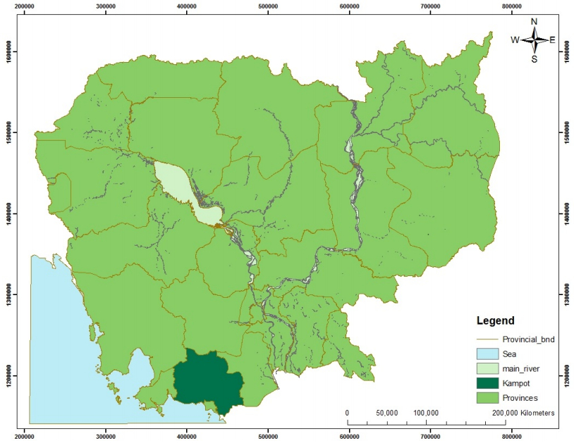
    [17] USAID (2010) Kampot Investment Profile.
    [18] Wang H, Velarde O, Bona S, et al. (2012) Patterns of varietal adoption and economics of rice production in Asia. Wang H, Pandey S, Velarde O, et al (eds). International Rice Res Institute.
    [19] Parry ML, Carter TR, Konijn NT (1988) The impact of climatic variation on agriculture. Vol 2: Assessments of semi-arid region. JAS 113: 281-284.
    [20] Lobell DB, Burke MB (2010) On the use of statistical models to predict crop yield responses to climate change. Agric For Meteorol 150: 1443-1452. doi: 10.1016/j.agrformet.2010.07.008
    [21] Hughes L (2000) Biological consequences of global warming: Is the signal already apparent? Trends Ecol Evol 15: 56-61. doi: 10.1016/S0169-5347(99)01764-4
    [22] Vouillamoz JM, Valois R, Lun S, et al. (2016) Can groundwater secure drinking-water supply and supplementary irrigation in new settlements of North-West Cambodia? Hydrogeol J 24: 195-209. doi: 10.1007/s10040-015-1322-6
    [23] Pheav S, Seng V, Reyes R, et al. (2003) Characterization of the Soil at the Stung Chinit Irrigation and Rural Infrastructure Project (SCIRIP). A final report submitted to GRET-CEDAC Stung Chinit project, Kampong Thom, Cambodia.
    [24] Meehl GA, Stocker TF, Collins WD, et al. (2007). Global Climate Projections. Solomon S, Qin D, Manning M, et al. (2007) (Eds). Cambridge University Press, Cambridge, UK. And New York NY.
    [25] Hatfield JL, Prueger JH (2015). Temperature extremes: effects of plant growth and development. Weather. Clim Extremes 10: 4-10. doi: 10.1016/j.wace.2015.08.001
    [26] Krishnan P, Ramakrishnan B, Reddy KR, et al. (2011). High-temperature effects on rice growth, yield, and grain quality. In: Advances in Agronomy (Sparks DL, eds). Burlington: Academic Press, 111: 87-206.
  • This article has been cited by:

    1. Mingzhou Xu, Complete convergence of moving average processes produced by negatively dependent random variables under sub-linear expectations, 2023, 8, 2473-6988, 17067, 10.3934/math.2023871
    2. Mingzhou Xu, Xuhang Kong, Complete qth moment convergence of moving average processes for m-widely acceptable random variables under sub-linear expectations, 2024, 214, 01677152, 110203, 10.1016/j.spl.2024.110203
    3. Mingzhou Xu, Kun Cheng, Wangke Yu, Convergence of linear processes generated by negatively dependent random variables under sub-linear expectations, 2023, 2023, 1029-242X, 10.1186/s13660-023-02990-6
    4. Mingzhou Xu, On the complete moment convergence of moving average processes generated by negatively dependent random variables under sub-linear expectations, 2024, 9, 2473-6988, 3369, 10.3934/math.2024165
    5. Mingzhou Xu, Complete convergence and complete moment convergence for maximal weighted sums of extended negatively dependent random variables under sub-linear expectations, 2023, 8, 2473-6988, 19442, 10.3934/math.2023992
    6. Lunyi Liu, Qunying Wu, Complete integral convergence for weighted sums of negatively dependent random variables under sub-linear expectations, 2023, 8, 2473-6988, 22319, 10.3934/math.20231138
    7. Yuyan Wei, Xili Tan, Peiyu Sun, Shuang Guo, Weak and strong law of large numbers for weakly negatively dependent random variables under sublinear expectations, 2025, 10, 2473-6988, 7540, 10.3934/math.2025347
  • Reader Comments
  • © 2017 the Author(s), licensee AIMS Press. This is an open access article distributed under the terms of the Creative Commons Attribution License (http://creativecommons.org/licenses/by/4.0)
通讯作者: 陈斌, bchen63@163.com
  • 1. 

    沈阳化工大学材料科学与工程学院 沈阳 110142

  1. 本站搜索
  2. 百度学术搜索
  3. 万方数据库搜索
  4. CNKI搜索

Metrics

Article views(5697) PDF downloads(1099) Cited by(10)

Figures and Tables

Figures(2)  /  Tables(6)

/

DownLoad:  Full-Size Img  PowerPoint
Return
Return

Catalog