Assessment of irrigation shortfall using WATHNET in the Otago region of New Zealand

Shailesh Kumar Singh; Richard Ibbitt; Shailesh Kumar Singh; Richard Ibbitt

doi:10.3934/geosci.2018.3.166

AIMS Geosciences

2018, Volume 4, Issue 3: 166-179. doi: 10.3934/geosci.2018.3.166

Previous Article Next Article

Research article

Assessment of irrigation shortfall using WATHNET in the Otago region of New Zealand

Shailesh Kumar Singh ^,,
Richard Ibbitt

National Institute of Water and Atmospheric Research, Christchurch, New Zealand

Received: 15 May 2018 Accepted: 04 September 2018 Published: 11 September 2018

Knowledge of the likely rainfall and river flow for a coming season can improve management of an overall water resources system without unduly compromising either the environmental or productive behaviour of the system. The objective of this study has been to assess the probability of irrigation demand shortfalls, i.e. soil moisture deficits, for a typical “run of the river” irrigation scheme so as to identify the duration and severity of potential shortfalls. In this study a multi-objective linear programming tool WATHNET has been used to build and run a model of the irrigation scheme. The focus of this study has been on how to use predictions of 3-monthly rainfall and temperature to estimate potential daily water available for irrigation. The method uses Monte-Carlo simulations, to produce multiple replicates of equally likely sequences of river flows, rainfall and potential evaporation values. A sub-set of the equally likely sequences is then selected using prediction information of the likely seasonal climate outlook from NIWA’s Climate Update. The selected sequences, which are biased towards the seasonal climate prediction, are then used as inputs to multiple model runs. By using the output from all the “biased” model runs a probability distribution can be made of water availability for irrigation. The methodology has been demonstrated using the Shag River Irrigation Scheme located in the Otago region of New Zealand. The results compare the predicted soil moisture variation over two three-month periods with retrospective simulations based on the observed rainfalls, river flows and potential evaporation values. Results suggest that WATHNET can simulate 3-month soil moisture dynamics. In order to develop WATHNET as a tool to assess probabilities of irrigation shortfall it needs to be validated using measurements of soil moisture variations over an irrigation season at sites with different soil types.

Keywords:

Citation: Shailesh Kumar Singh, Richard Ibbitt. Assessment of irrigation shortfall using WATHNET in the Otago region of New Zealand[J]. AIMS Geosciences, 2018, 4(3): 166-179. doi: 10.3934/geosci.2018.3.166

Related Papers:

[1]	Zhiyan Ding, Hichem Hajaiej . On a fractional Schrödinger equation in the presence of harmonic potential. Electronic Research Archive, 2021, 29(5): 3449-3469. doi: 10.3934/era.2021047
[2]	Yixuan Wang, Xianjiu Huang . Ground states of Nehari-Pohožaev type for a quasilinear Schrödinger system with superlinear reaction. Electronic Research Archive, 2023, 31(4): 2071-2094. doi: 10.3934/era.2023106
[3]	Jiayi Fei, Qiongfen Zhang . On solutions for a class of Klein–Gordon equations coupled with Born–Infeld theory with Berestycki–Lions conditions on $\mathbb{R}^3$ . Electronic Research Archive, 2024, 32(4): 2363-2379. doi: 10.3934/era.2024108
[4]	Xiaoyong Qian, Jun Wang, Maochun Zhu . Existence of solutions for a coupled Schrödinger equations with critical exponent. Electronic Research Archive, 2022, 30(7): 2730-2747. doi: 10.3934/era.2022140
[5]	Senli Liu, Haibo Chen . Existence and asymptotic behaviour of positive ground state solution for critical Schrödinger-Bopp-Podolsky system. Electronic Research Archive, 2022, 30(6): 2138-2164. doi: 10.3934/era.2022108
[6]	Xiaoguang Li . Normalized ground states for a doubly nonlinear Schrödinger equation on periodic metric graphs. Electronic Research Archive, 2024, 32(7): 4199-4217. doi: 10.3934/era.2024189
[7]	Xincai Zhu, Yajie Zhu . Existence and limit behavior of constraint minimizers for elliptic equations with two nonlocal terms. Electronic Research Archive, 2024, 32(8): 4991-5009. doi: 10.3934/era.2024230
[8]	Hui Jian, Min Gong, Meixia Cai . Global existence, blow-up and mass concentration for the inhomogeneous nonlinear Schrödinger equation with inverse-square potential. Electronic Research Archive, 2023, 31(12): 7427-7451. doi: 10.3934/era.2023375
[9]	Xian Zhang, Chen Huang . Existence and multiplicity of sign-changing solutions for supercritical quasi-linear Schrödinger equations. Electronic Research Archive, 2023, 31(2): 656-674. doi: 10.3934/era.2023032
[10]	Xiaoju Zhang, Kai Zheng, Yao Lu, Huanhuan Ma . Global existence and long-time behavior of solutions for fully nonlocal Boussinesq equations. Electronic Research Archive, 2023, 31(9): 5406-5424. doi: 10.3934/era.2023274

Abstract

1. Introduction

Cycling has been considered as one of the most popular sports around the world. The major concern about cyclist's performance is to reach their averaged maximal speed as soon as possible and maintain it over a race. According to Newton's second law (equation 1), acceleration is given by the ration between force and mass (equation 2). Knowing that, cyclists propulsion may overcome the resistance (equation 3) [1].

$F = m . a$ (1)

Where, F is the force, m the mass and a is the acceleration.

$a = \frac{F}{m}$ (2)

$a = \frac{(F_{p r o p} + F_{r e s})}{m}$ (3)

Where, F_prop are the propulsive forces and F_res the resistive forces in negative direction of the motion.

Cyclists aim to improve performance minimizing the winning time and effort during the race. To maintain the averaged speed, cyclists may deliver energy to the pedals. Among the delivered energy by the cyclist, some is necessary to overcome resistance and other lost by the bicycle-cyclist system.

$v = \sqrt{\frac{2 (ϵ_{i n} - ϵ_{l o s s})}{m}}$ (4)

Some strategies are adopted to reduce the required energy at a given speed or pace. Cyclists used to wear different helmets and adopt different body positions on the bicycle to minimize resistance [2],[3]. Drag is the main resistive force in cycling and contributes about 90% of the resistance [4]–[6]. Among the different positions (normal, dropped and aero), there is the drooped position [7]. This position aims to reduce frontal surface area and drag in comparison to the normal position [7]. Moreover, it is dependent of anthropometrics, trunk position and bicycle control in the different road curves and slopes; whereas the aero position is mainly used in straight events [8]–[11].

Drag can be assessed by analytical procedures, coasting deceleration methods, wind tunnel testing and numerical simulations by computer fluid dynamics (CFD) [12]. However, CFD has been used to understand the fluid flow behavior around an object [12],[13]. This methodology helps to control confounding factors such as temperature, side winds or assumptions such as drag coefficient. Wind tunnel testing is considered the gold standard method; however, the tests are expensive and demand a considered time consumption [12]. The analytical procedures required a set of assumptions and estimations and coasting technics do not allow to control environmental conditions [12].

Helmets designs aim to improve cyclists performance, reducing the winning time. Upon the different helmets type, a so called: (i) standard and; (ii) aero road helmet. This new aero road helmets are characterized by different tail lengths and reduced air vents, intending to improve efficiency and aerodynamics [3],[14],[15]. Recently, elite road cyclists have been using these “new” aero road helmets due the impossibility to use time-trial helmets in track races. That might be related with the importance of minimize drag and improve efficiency, as in time-trial helmets [3]. However, it is yet unclear what is the effect of these new type of helmets on a rider's aerodynamics.

To date, this is the first attempt that this new type of helmets is tested in the dropped position. Moreover, most studies with helmets are made in the aero position or only assess the helmet. Thus, the aim of this study was to compare a standard helmet with the new aero road helmets in a bicycle-cyclist system by CFD. It was hypothesized that the aero road helmet imposes a lower drag in the bicycle/cyclist system.

2. Materials and method

2.1. Subject

An elite level road cyclist, racing regularly at national level events volunteered to this research. The bicycle-cyclist system mass was 62 kg (cyclist: 55.0 kg of body mass and 1.76 m of height). All procedures were in accordance to the Helsinki Declaration regarding human research and a written consent was obtained beforehand.

2.2. Scanning the model

The cyclist was scanned on his racing bicycle on the dropped position wearing competition gear and each of the two helmets. The scans were wearing a standard helmet (Figure 1 at left; Giant, Rev Helmet) and an aero road helmet (Figure 1 at right; Giant, Pursuit Helmet) (Figure 1). The Rev Helmet type pull the incoming air from the front and side channels to back; whereas the Pursuit Helmet aims to produce the wind-cheating effects of time-trial helmets to the road without sacrificing ventilation with only two ventilation channels (front and back).

The scanning process was made with a Sense 3D scanner (3D Systems, Inc., Canada) and saved in the Sense Software (Sense, 3D Systems, Inc., Canada). The scanner precision was 0.0009 m (0.9 mm) at 0.5 m (50 cm) distance. The Sense software allowed to clean, fill holes and solidify the geometry, then the model was exported as stereolithographic file (.stl). The Geomagic studio (3D Systems, USA) was used to edit and post process the geometry in stl format. The models were meshed, smoothed, clean self-intersections, spikes and non-manifold edges on Geomagic studio. CAD models were created from the geometries [13] (Figure 1).

Figure 1. Three-dimensional models of the cyclist on the dropped position with a standard (left) and an aero road helmet (right).

DownLoad: Full-Size Img PowerPoint

2.3. Boundary conditions

In Ansys Workbench software (Ansys Fluent 16.0, Ansys Inc., Pennsylvania, USA) the models were imported to start the numerical simulations process. The boundary dimensions were created in the geometry module with a three-dimensional domain around the cyclist with 7 m of length, 2.5 m of width and 2.5 m of height (Figure 2). The domain was meshed to represent the fluid flow in the opposite direction to the cyclist with more than 43 million of prismatic and tetrahedral elements and the cell size were near 25.72 µm and (Ansys Mesh, Ansys Inc., Pennsylvania, USA). The cyclist was placed at 2.5 meters of the inlet portion [16].

Figure 2. Three-dimensional domain of the cyclist on the dropped position with a standard helmet.

DownLoad: Full-Size Img PowerPoint

During a race, the mean speed is about 11.1 m/s (∼ 40 km/h) [17]. The velocity was set at the inlet portion of the enclosure surface (-z direction) at 11.1 m/s (∼ 40 km/h). The turbulence intensity was assumed as 1×10^−6%. The bicycle-cyclist system surface was established as zero roughness, non-slip wall and scalable wall functions were assigned.

2.4. Numerical simulations

The Fluent CFD code (Ansys Fluent 16.0, Ansys Inc., Pennsylvania, USA) run the Reynolds-averaged Navier–Stokes (RANS) equations (equations 5, 6, 7 and 8) and assess the fluid flow behavior (equation 5), Reynolds Stresses (equation 6), temperature (equation 7) and mass transfer (equation 8). The RANS equations transform instantaneous values into means. Fluent CFD code (Ansys Fluent 16.0, Ansys Inc., Pennsylvania, USA) solve these equations by the finite volume approach. The Realizable k-e was selected as the turbulence model where the velocity histograms are very similar to the standard k-e, RST and RNG k-e models [18]. The standard wall function was selected for this simulation.

$\frac{\partial U_{i}}{\partial x_{i}} = 0$ (5)

$\frac{\partial U_{i}}{\partial_{t}} \pm U_{j} \frac{\partial U_{i}}{\partial x_{j}} = - \frac{1}{ρ} \frac{\partial P}{\partial x_{j}} + \frac{\partial}{\partial x_{j}} (2 v S_{i j} - \bar{μ_{j}^{'} μ_{i}^{'}})$ (6)

$\frac{\partial θ_{i}}{\partial_{t}} \pm U_{j} \frac{\partial θ}{\partial x_{j}} = \frac{1}{ρ c_{p}} \frac{\partial}{\partial x_{j}} (k \frac{\partial θ}{\partial x_{j}} - \bar{μ_{j}^{'} θ^{'}})$ (7)

$\frac{\partial C}{\partial t} \pm U_{j} \frac{\partial C}{\partial x_{j}} = \frac{\partial}{\partial x_{j}} (D \frac{\partial C}{\partial x_{j}} - \bar{μ_{j}^{'} c^{'}})$ (8)

Where, U_i and x_i are the instantaneous velocity and the position, p the instantaneous pressure, t is the time, ρ the fluid density, v is the molecular kinematic viscosity, c_p heat capacity, k is the thermal conductivity and S_ij the strain-rate tensor, c is the instantaneous concentration, and D is the molecular diffusion coefficient. The Reynolds stresses component ( $\bar{μ_{j}^{'} μ_{i}^{'}}$ ), describes the turbulence of the mean flow being the exchange of momentum by the change of the fluid parcels. The Reynolds stress is given by:

$\bar{μ_{j}^{'} μ_{i}^{'}} = 2 v_{t} S_{i j} - \frac{2}{3} T K E δ_{i j}$ (9)

Where, v_t is the turbulent viscosity and the mean strain rate S_ij is given by,

$S_{i j} = \frac{1}{2} (\frac{\partial U_{i}}{\partial_{x j}} + \frac{\partial j}{\partial_{x i}})$ (10)

The turbulent kinetic energy (TKE) is given by,

$T K E = \frac{1}{2} \bar{μ_{i}^{'} μ_{i}^{'}}$ (11)

And the kronecker delta (δ_ij),

$δ_{i j} = {\begin{matrix} 1; i f i = j \\ 0; i f i \neq j \end{matrix}$ (12)

The SIMPLE algorithm was used for pressure–velocity coupling. The pressure interpolation and the convection and viscous terms of the governing equations discretization schemes were defined as second. The least-squares cell-based method computed the gradients. Pressure and momentum were defined as second order and second order upwind and the turbulent kinetic energy and turbulent dissipation rate as first order upwind. The convergence occurred automatically by the Ansys Fluent 16.0 (Ansys Fluent 16.0, Ansys Inc., Pennsylvania, USA) before 1,404 interactions.

2.5. Outcomes

After the numerical simulations, outputs such as viscous, pressure, total drag and coefficient of drag are possible to obtain. Ansys Fluent Software (Ansys Fluent 16.0, Ansys Inc., Pennsylvania, USA) computed the surface area.

To compute the drag force, equation (13) was used:

$F_{d} = \frac{1}{2} ρ A C_{d} v^{2}$ (13)

Where, F_d is the drag force, C_d represents the drag coefficient, v the velocity, A the surface area and ρ is the air density (1.292 kg/m³).

Pressure coefficient (Cp) and relative velocity magnitude (m/s) graphical representation were obtained in Ansys Fluent 16.0 (Ansys Fluent 16.0, Ansys Inc., Pennsylvania, USA) after the numerical simulations. The contours of pressure and velocity were obtained without filled geometries.

3. Results

The aero road helmet presented a lower viscous, pressure and total drag in comparison to the standard helmet (Figure 3). The standard helmet presented a viscous drag of 10.52 N and the aero road helmet 7.40 N. The pressure drag of the standard helmet was 16.51 N for the selected speed and 12.56 N for the aero road helmet. Moreover, the total drag of the standard helmet was 21.98 N and the aero road helmet was 19.96 N.

Figure 3. Viscous, pressure and total drag at 11.11 m/s for the standard and aero helmet.

DownLoad: Full-Size Img PowerPoint

The aero road helmet presented a lower viscous, pressure and total drag coefficient in comparison to the standard helmet (Figure 4). The standard helmet presented a viscous drag coefficient of 0.30 and the aero road helmet 0.21. The standard helmet pressure drag coefficient was 0.46 N for the selected speed and 0.35 for the aero road helmet. The total drag coefficient of the standard helmet was 0.76 and the aero road helmet was 0.56.

Figure 4. Viscous, pressure and total drag coefficient at 11.11 m/s for the standard and aero helmet.

DownLoad: Full-Size Img PowerPoint

The aero road helmet a lower pressure coefficient (Cp) in comparison to the standard helmet (Figure 5). The standard helmet presented a Cp between −3.94 and 1.08; whereas the aero road helmet presented a Cp between −3.63 and 1.05.

Figure 5. Coefficient of Pressure for standard helmet (left) and aero road helmet (right) at 11.11 m/s.

DownLoad: Full-Size Img PowerPoint

The aero road helmet presented a lower relative velocity magnitude (m/s) in comparison to the standard helmet (Figure 6). The relative velocity magnitude for the standard helmet ranged between 3.11x10⁻³ and 22.24 m/s. The relative velocity magnitude for the aero road helmet ranged between 2.87x10⁻³ and 22.2 m/s.

Figure 6. Relative velocity magnitude in (m/s) for standard helmet (left) and aero road helmet (right) at 11.11 m/s.

DownLoad: Full-Size Img PowerPoint

4. Discussions

The aim of this study was to assess the aerodynamics of an elite cyclist wearing a standard and an aero road helmet on the dropped position by computer fluid dynamics. The main results were that the aero road helmet presented lower viscous, pressure and total drag, such as viscous, pressure and total drag coefficient.

An elite level cyclist volunteered for this research. Aerodynamic analysis by CFD are usually made with elite subjects, representatives of the sport [3],[4],[13]. Cyclist's averaged speed in tours is near 11.11 m/s (≈ 40 km/h) [17]. This was the selected speed to assess drag in our study. Moreover, during a race, the dropped position is one of the adopted positions to minimize drag in comparison to the normal position [7]. In our study, the dropped position was the selected position. The numerical simulations by CFD has been used to assess cyclists drag in different situations [12],[13]. CFD presented concordance with wind tunnel experiments [7],[19],[20].

The standard helmet imposed a higher drag in comparison to the aero road helmet. The standard helmet total was 21.98 N and the aero road helmet 19.96 N. Forte et al. [21], compared a standard and an aero helmet at wheelchair racing speeds (maximal 6.5 m/s). The differences between helmets were near 30%. However, the authors only evaluated the head and helmet. In our study, the bicycle-cyclist system was assessed with the different helmets and the total drag differences was 9%. The differences magnitude might be explained by: (i) the selected speeds were different; (ii) the fluid flow around the bicycle-cyclist geometry was different from the head and helmet. Brownlie et al. [22], also reported that time trial helmets reduce the cyclists drag. These findings seem to be in accordance with our study. The drag coefficient with the standard helmet was 0.76 and the aero road helmet was 0.56. The drag coefficient is dependent of the geometry form or shape [23],[24]. Moreover, the fluid flow between helmets may also explain the drag coefficient changes [23]–[25]. In our study, the difference between the two helmets in drag coefficient was 26%. In Beaumont et al. [3] study, the drag coefficient differences between three helmets were about 3.1%. However, the authors only assessed drag with the cyclist body and the bicycle was not included in the analysis. In our study, the pressure coefficient was slightly higher in the standard helmet in comparison to the aero road helmet. The same phenomenon was observed in the relative velocity magnitude between helmets. The reduced air vents might also explain the differences between the helmets. Helmets with smooth surfaces are designed by engineers and sports scientists to minimize drag coefficient [3],[14],[15]. This may also contribute to reduce parasite turbulence and drag [26].

Overall, the pressure coefficient and relative velocity magnitude did not presented an accentuated difference. This is supported by the Blocken et al. study [7], the authors reported Cp near -1 and 1. In our study, the highest Cp was 1.08. This may suggest that the drag differences were due the fluid flow around bicycle-cyclist geometries with the different helmets [21], [23]–[26]. In our study, the selected aero road helmet presented less air vents and drag coefficient in comparison to the standard type. Upon that, cycling practitioners may choose to use aero road helmets type with reduce air vents to produce the wind-cheating effects of time-trial helmets instead of normal helmets with front/side and back air channels.

The present study present the following limitations: (i) only one position was assessed; (ii) the cyclist spent more time in the normal position than in the dropped position; (iii) numerical simulations were only performed at one speed; (iv) different temperatures were not tested; (v) the cyclist was only representative of elite level, so results might not be extrapolated to others. It can be addressed as further research: (i) comparisons between more helmets types; (ii) design and customize a specific helmet for the athlete; (iii) assess drag with different temperatures and positions; (iv) evaluate active drag by numerical simulations.

5. Conclusions

It is possible to conclude that an aero road helmet imposes less drag in comparison to a standard helmet. Thus, coaches should advise their athletes to use aero road helmets during a race. The resistance acting on an elite cyclist in the dropped position was higher with a standard helmet than with an aero road helmet.

References

[1]	Davids Engineering I (2015) Solano Irrigation District Water Supply Shortage Risk Assessment, Available from: https://www.sidwater.org/documentcenter/view/998.
[2]	Zotarelli L, Dukes M, Morgan K (2010) Interpretation of soil moisture content to determine soil field capacity and avoid over-irrigating sandy soils using soil moisture sensors. University of Florida Cooperation Extension Services, AE460.
[3]	Oweis T, Hachum A (2006) Water harvesting and supplemental irrigation for improved water productivity of dry farming systems in West Asia and North Africa. Agr Water Manage 80: 57–73. doi: 10.1016/j.agwat.2005.07.004
[4]	Singh SK (2016) Long-term Streamflow Forecasting Based on Ensemble Streamflow Prediction Technique: A Case Study in New Zealand. Water Resour Manage 30: 2295–2309. doi: 10.1007/s11269-016-1289-7
[5]	Kuczera G, Cui L, Gilmore R, et al. (2009) Addressing the shortcomings of water resource simulation models based on network linear programming. 32nd Hydrology and Water Resources Symposium (H2009). Newcastle, Australia Engineers Australia/Causal Productions.
[6]	Singh SK, Williams G, Ibbitt R (2016) Opeartional and strategic planning for dynamic water supply system. Water New Zealand's Annual Conference & Expo, 19–21 Oct Rotorua, New Zealand.
[7]	Singh S, Ibbitt R, Mullan B (2016) Sustainable Yield Model Upgrade 2016: SYM Upgrade 2016. Wellington Water Ltd (Working on behalf of the Greater Wellington Regional Council), 85.
[8]	Ibbitt RP (2004) KARAKA model: A seasonal water availability model based on the SYM. WRC05501. Christchurch: NIWA, 57: 57 figs, 51 table.
[9]	Kuczera G, Cui L, Gilmore R, et al. (2010) Enhancing the robustness of water resource simulation models based on network linear programming. 9th International conference on Hydroinformatics. Tianjin, China: Chemical Industry Press (CIP), 2245–2252.
[10]	Cui L, Ravalico J, Kuczera G, et al. (2011) Multi-onjective Optimisation Methodology for the Canberra Water Supply System. Canberra, Australia: eWater Cooperative Research Centre.
[11]	Mortazavi M, Kuczera G, Cui L (2012) Multiobjective optimization of urban water resources: Moving toward more practical solutions. Water Resour Res 48.
[12]	Mortazavi-Naeini M, Kuczera G, Kiem AS, et al. (2013) Robust optimisation of urban drought security for an uncertain climate. National Climate Change Adaptation Research Facility Gold Coast, 74.
[13]	Fahey B, Ekanayake J, Jackson R, et al. (2010) Unisg the WATYIELD water balance model to predict catchmnet water yields and low flows. J Hydrol 49: 35–58.
[14]	Ibbitt RP (2005) Otago Strategic Water Study: 1. Natural flow series and water availability for eight catchments. ORC05503. Christchurch: NIWA, 96: 146 figs, 144 tables, 145 refs.
[15]	UKWIR (2002) An Improved Methodology for Assessing Headroom. ReportWR-13, UK Water Industry Research Ltd, London.
[16]	Ibbitt RP, Woolley K (2008) Seasonal prediction of supply and demand for a dynamic water supply system. 16–18 October Bangkok.
[17]	Ibbitt RP (1997) Documentation for the Reliable Yield Model for the bulk water supply system for the Wellington Regional Council. WRC70501. Christchurch: NIWA, 3 v.: ill. (some missing) tables, refs.
[18]	Varley I (2016) WATHNET Water Supply System Model Independent Review 2016-Final report, WaterNSW, WR2016-002J, Available from: https://www.waternsw.com.au/__data/assets/pdf_file/0019/73504/Wathnet-Water-Supply-System-Model-Independent-Review-2016.PDF.
[19]	SKM, Water Supply System Model and Yield Review 2009/2010, Volume 1: Main Report, 2011. Available from: https://www.waternsw.com.au/__data/assets/pdf_file/0003/55929/WSSMYieldReview2010Vol1.pdf.
[20]	Bandaragoda C, Tarboton DG, Woods R (2004) Application of TOPNET in the distributed model intercomparison project. J Hydrol 298: 178–201. doi: 10.1016/j.jhydrol.2004.03.038
[21]	Ibbitt RP, Woods RA, McKerchar AI (2004) Otago Strategic Water Study: 1. Natural flow series and water availability for eight catchments-Draft. Christchurch: NIWA, 72 leaves: 152 figs, 153 tables, 153 refs.
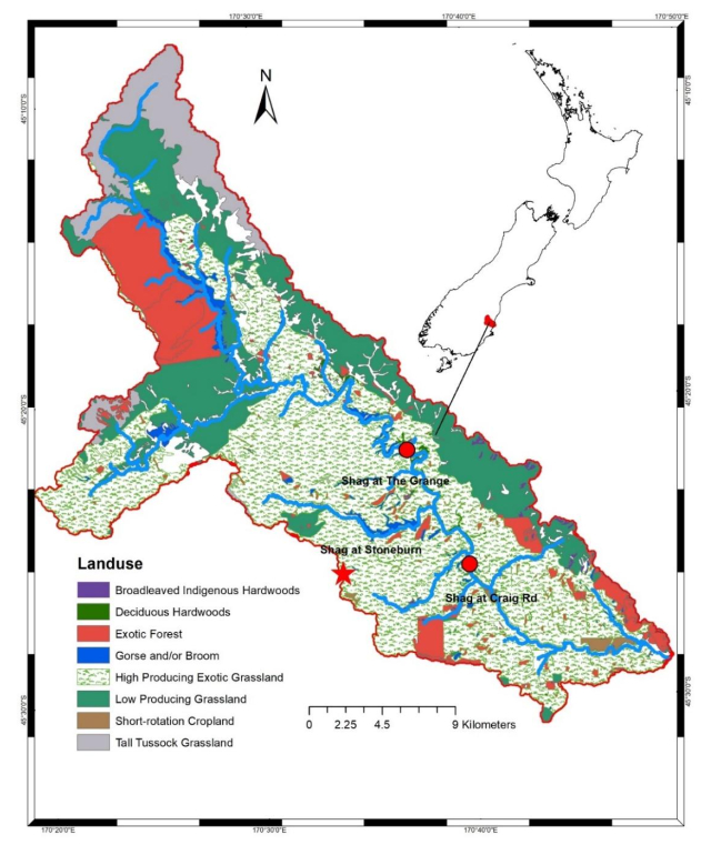
[22]	ORC, Flow at Shag River, 2018. Available from: http://water.orc.govt.nz/WaterInfo/Site.aspx?s=ShagGrange, Accesed on 01 Feb 2018.

This article has been cited by:

1.	Pedro Forte, Daniel A. Marinho, Pantelis T. Nikolaidis, Beat Knechtle, Tiago M. Barbosa, Jorge E. Morais, Analysis of Cyclist’s Drag on the Aero Position Using Numerical Simulations and Analytical Procedures: A Case Study, 2020, 17, 1660-4601, 3430, 10.3390/ijerph17103430
2.	Pedro Forte, Jorge E. Morais, Henrique P. Neiva, Tiago M. Barbosa, Daniel A. Marinho, The Drag Crisis Phenomenon on an Elite Road Cyclist—A Preliminary Numerical Simulations Analysis in the Aero Position at Different Speeds, 2020, 17, 1660-4601, 5003, 10.3390/ijerph17145003
3.	Pedro Forte, Jorge E. Morais, Tiago M. Barbosa, Daniel A. Marinho, Assessment of Able-Bodied and Amputee Cyclists’ Aerodynamics by Computational Fluid Dynamics, 2021, 9, 2296-4185, 10.3389/fbioe.2021.644566
4.	Daniel A. Marinho, Dennis Willemsen, Tiago M. Barbosa, António José Silva, J. Paulo Vilas-Boas, Henrique P. Neiva, Pedro Forte, Numerical simulations of a swimmer’s head and cap wearing different types of goggles, 2021, 1476-3141, 1, 10.1080/14763141.2021.1923793

Reader Comments

Your name:*

Email:*
© 2018 the Author(s), licensee AIMS Press. This is an open access article distributed under the terms of the Creative Commons Attribution License (http://creativecommons.org/licenses/by/4.0)

通讯作者: 陈斌, bchen63@163.com

1.
沈阳化工大学材料科学与工程学院沈阳 110142

AIMS Geosciences

0.9

Metrics

Article views(3822) PDF downloads(726) Cited by(1)

Preview PDF

Download XML

Export Citation

Article outline

Show full outline

AIMS Geosciences

Assessment of irrigation shortfall using WATHNET in the Otago region of New Zealand

Related Papers:

Abstract

1. Introduction

2. Materials and method

2.1. Subject

2.2. Scanning the model

2.3. Boundary conditions

2.4. Numerical simulations

2.5. Outcomes

3. Results

4. Discussions

5. Conclusions

References

This article has been cited by:

Reader Comments

通讯作者: 陈斌, bchen63@163.com

Metrics

Figures and Tables

Other Articles By Authors

Catalog

Abstract

1. Introduction

2. Materials and method

2.1. Subject

2.2. Scanning the model

2.3. Boundary conditions

2.4. Numerical simulations

2.5. Outcomes

3. Results

4. Discussions

5. Conclusions

References

AIMS Geosciences

Assessment of irrigation shortfall using WATHNET in the Otago region of New Zealand

Related Papers:

Abstract

1. Introduction

2. Materials and method

2.1. Subject

2.2. Scanning the model

2.3. Boundary conditions

2.4. Numerical simulations

2.5. Outcomes

3. Results

4. Discussions

5. Conclusions

References

This article has been cited by:

Reader Comments

通讯作者: 陈斌, bchen63@163.com

Metrics

Figures and Tables

Other Articles By Authors

Related pages

Tools

Export File

Citation

Format

Content

Catalog

Abstract

1. Introduction

2. Materials and method

2.1. Subject

2.2. Scanning the model

2.3. Boundary conditions

2.4. Numerical simulations

2.5. Outcomes

3. Results

4. Discussions

5. Conclusions

References