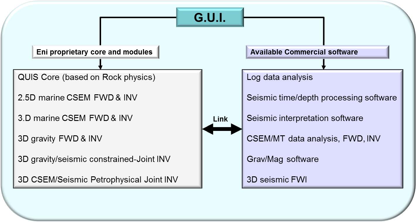
This paper reviews the theoretical aspects and the practical issues of different types of geophysical integration approaches. Moreover it shows how these approaches can be combined and optimized into the same platform. We discuss both cooperative modeling and Simultaneous Joint Inversion (SJI) as complementary methods for integration of multi-domain geophysical data: these data can be collected at surface (seismic, electromagnetic, gravity) as well as in borehole (composite well logs). The main intrinsic difficulties of any SJI approach are the high computational requirements, the non-uniqueness of the final models, the proper choice of the relations between the different geophysical domains, the quantitative evaluation of reliability indicators. In order to face efficiently all these problems we propose and describe here a “systemic approach”: the algorithms of modeling and SJI are merged with an integration architecture that permits the selection of workflows and links between different algorithms, the management of data and models coming from different domains, the smart visualization of partial and final results. This Quantitative Integration System (QUIS) has been implemented into a complex software and hardware platform, comprising many advanced codes working in cooperation and running on powerful computer clusters. The paper is divided into two main parts. First we discuss the theoretical formulation of SJI and the key concepts of the QUIS platform. In the second part we present a synthetic SJI test and a case history of QUIS application to a real exploration problem.
Citation: Dell’Aversana Paolo, Bernasconi Giancarlo, Chiappa Fabio. A Global Integration Platform for Optimizing Cooperative Modeling and Simultaneous Joint Inversion of Multi-domain Geophysical Data[J]. AIMS Geosciences, 2016, 2(1): 1-31. doi: 10.3934/geosci.2016.1.1
This paper reviews the theoretical aspects and the practical issues of different types of geophysical integration approaches. Moreover it shows how these approaches can be combined and optimized into the same platform. We discuss both cooperative modeling and Simultaneous Joint Inversion (SJI) as complementary methods for integration of multi-domain geophysical data: these data can be collected at surface (seismic, electromagnetic, gravity) as well as in borehole (composite well logs). The main intrinsic difficulties of any SJI approach are the high computational requirements, the non-uniqueness of the final models, the proper choice of the relations between the different geophysical domains, the quantitative evaluation of reliability indicators. In order to face efficiently all these problems we propose and describe here a “systemic approach”: the algorithms of modeling and SJI are merged with an integration architecture that permits the selection of workflows and links between different algorithms, the management of data and models coming from different domains, the smart visualization of partial and final results. This Quantitative Integration System (QUIS) has been implemented into a complex software and hardware platform, comprising many advanced codes working in cooperation and running on powerful computer clusters. The paper is divided into two main parts. First we discuss the theoretical formulation of SJI and the key concepts of the QUIS platform. In the second part we present a synthetic SJI test and a case history of QUIS application to a real exploration problem.

| [1] |
Abubakar A., Li M., Pan G., Liu J., Habashy T.M. (2011) Joint MT and CSEM data inversion using a multiplicative cost function approach. Geophysics 76: F203-F214. doi: 10.1190/1.3560898

|
| [2] |
Colombo D., De Stefano (2007) M., Geophysical modeling via simultaneous joint inversion of seismic, gravity, and electromagnetic data. The Leading Edge 26: 326-331. doi: 10.1190/1.2715057
|
| [3] | Colombo D., Mantovani M., DeStefano M., Garrad D., Al Lawati H. (2007) Simultaneous Joint Inversion of Seismic and Gravity data for long offset Pre-Stack Depth Migration in Northern Oman, CSEG, Calgary. |
| [4] |
Commer M., Newman G.A. (2009) Three-dimensional controlled-source electromagnetic andmagnetotelluric joint inversion. Geophys. J. Int 178: 1305-1316. doi: 10.1111/j.1365-246X.2009.04216.x
|
| [5] |
Constable S., Srnka L. (2007) An introduction to marine controlled-source electromagnetic methods for hydrocarbon exploration. Geophysics 72: WA3-WA12. doi: 10.1190/1.2432483
|
| [6] | Dell’Aversana P., Zanoletti F. (2010) Spectral analysis of marine CSEM data symmetry. First Break 28: 44-51. |
| [7] |
Dell’Aversana P., Bernasconi G., Miotti F., Rovetta D. (2011) Joint inversion of rock properties from sonic, resistivity and density well-log measurements. Geophysical Prospecting 59: 1144-1154. doi: 10.1111/j.1365-2478.2011.00996.x
|
| [8] | Dell’Aversana P., Colombo S., Ciurlo B., Leutscher J., Seldal J. (2012) CSEM data interpretation constrained by seismic and gravity data. An application in a complex geological setting. First Break 30: 35-44. |
| [9] | Dell’Aversana P. (2014) Integrated Geophysical Models: Combining Rock Physics with Seismic, Electromagnetic and Gravity Data. EAGE Publications . |
| [10] |
DeStefano M., Golfré Andreasi F., Re S., Virgilio M., Snyder F.F. (2011) Multiple-domain, simultaneous joint inversion of geophysical data with application to subsalt imaging. Geophysics 76: R69. doi: 10.1190/1.3554652
|
| [11] | Eidesmo T., Ellingsrud S., MacGregor L.M., Constable S., Sinha M.C., Johansen S., Kong F.N., Westerdah H. (2002) Sea bed logging, a new method for remote and direct identification of hydrocarbon filled layers in deepwater areas. First Break 20: 144-152. |
| [12] |
Gallardo L.A., Meju M.A. (2003) Characterization of heterogeneous near-surface materials by joint 2D inversion of dc resistivity and seismic data. GEOPHYSICAL RESEARCH LETTERS 30: 1658. doi: 10.1029/2003GL017370
|
| [13] | Gallardo L.A., Meju M.A. (2004) Joint two-dimensional DC resistivity and seismic travel time inversion with cross-gradients constraints. J. geophys 109. |
| [14] |
Gallardo L.A., Meju M.A. (2007) Joint two-dimensional cross-gradient imaging of magnetotelluric and seismic traveltime data for structural and lithological classification. Geophys. J. Int. 169: 1261-1272. doi: 10.1111/j.1365-246X.2007.03366.x
|
| [15] |
Haber E., Oldenburg D.W (1997) Joint inversion: a structural approach. Inverse Problems 13: 63-77. doi: 10.1088/0266-5611/13/1/006
|
| [16] |
Hu W., Abubakar A., Habashy T.M. (2009) Joint electromagnetic and seismic inversion using structural constraints. Geophysics 74: R99-R109. doi: 10.1190/1.3246586
|
| [17] | Jin J. (2002) The Finite Element Method in Electromagnetics. John Wiley&Sons . |
| [18] | Kennett B.L.N. (1983) Seismic wave propagation in stratified media. Cambridge University Press . |
| [19] |
Liang L., Abubakar A., Habashy T.M. (2011) Estimating petrophysical parameters and average mud-filtrate invasion rates using joint inversion of induction logging and pressure transient data. Geophysics 76: E21-E34. doi: 10.1190/1.3541963
|
| [20] |
Moorkamp M., Heincke B., Jegen M., Roberts A.W., Hobbs R.W. (2011) A framework for 3-D joint inversion of MT, gravity and seismic refraction data. Geophys. J. Int 184: 477-493. doi: 10.1111/j.1365-246X.2010.04856.x
|
| [21] | Raymer L.L., Hunt E.R., Gardner J.S. (1980) An improved sonic transit time to porosity transform. 21st Annual Logging Symposium. Transactions of the Society of Professional Well Log Analysts P546. |
| [22] | Schön J.H. (2011) Physical Properties of Rocks: Fundamentals and Principles of Petrophysics. Elsevier . |
| [23] | Tarantola A. (2005) Inverse Problem Theory and Methods for Model Parameter Estimation. Society for Industrial and Applied Mathematics . |
| [24] |
Thomson W.T. (1950) Transmission of Elastic Waves through a Stratified Solid medium. Jour. Appl. Phys. 21: 89-93. doi: 10.1063/1.1699629
|
| [25] |
Vozoff K., Jupp D.L.B. (1975) Joint Inversion of Geophysical Data. Geophys. J 42: 977-991. doi: 10.1111/j.1365-246X.1975.tb06462.x
|


Figures(19) / Tables(4)

Dell’Aversana Paolo, Bernasconi Giancarlo, Chiappa Fabio. A Global Integration Platform for Optimizing Cooperative Modeling and Simultaneous Joint Inversion of Multi-domain Geophysical Data[J]. AIMS Geosciences, 2016, 2(1): 1-31. doi: 10.3934/geosci.2016.1.1


 DownLoad: