Stereo matching is still very challenging in terms of depth discontinuity, occlusions, weak texture regions, and noise resistance. To address the problems of poor noise immunity of local stereo matching and low matching accuracy in weak texture regions, a stereo matching algorithm (iFCTACP) based on improved four-moded census transform (iFCT) and a novel adaptive cross pyramid (ACP) structure were proposed. The algorithm combines the improved four-moded census transform matching cost with traditional measurement methods, which allows better anti-interference performance. The cost aggregation is performed on the adaptive cross pyramid structure, a unique structure that improves the traditional single mode of the cross. This structure not only enables regions with similar color and depth to be connected but also achieves cost smoothing across regions, significantly reducing the possibility of mismatch due to inadequate corresponding matching information and providing stronger robustness to weak texture regions. Experimental results show that the iFCTACP algorithm can effectively suppress noise interference, especially in illumination and exposure. Furthermore, it can markedly improve the error matching rate in weak texture regions with better generalization. Compared with some typical algorithms, the iFCTACP algorithm exhibits better performance whose average mismatching rate is only 3.33$ \% $.
Citation: Zhongsheng Li, Jianchao Huang, Wencheng Wang, Yucai Huang. A new stereo matching algorithm based on improved four-moded census transform and adaptive cross pyramid model[J]. Electronic Research Archive, 2024, 32(7): 4340-4364. doi: 10.3934/era.2024195
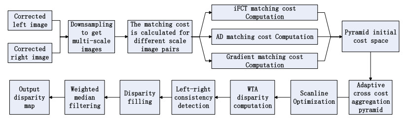
Stereo matching is still very challenging in terms of depth discontinuity, occlusions, weak texture regions, and noise resistance. To address the problems of poor noise immunity of local stereo matching and low matching accuracy in weak texture regions, a stereo matching algorithm (iFCTACP) based on improved four-moded census transform (iFCT) and a novel adaptive cross pyramid (ACP) structure were proposed. The algorithm combines the improved four-moded census transform matching cost with traditional measurement methods, which allows better anti-interference performance. The cost aggregation is performed on the adaptive cross pyramid structure, a unique structure that improves the traditional single mode of the cross. This structure not only enables regions with similar color and depth to be connected but also achieves cost smoothing across regions, significantly reducing the possibility of mismatch due to inadequate corresponding matching information and providing stronger robustness to weak texture regions. Experimental results show that the iFCTACP algorithm can effectively suppress noise interference, especially in illumination and exposure. Furthermore, it can markedly improve the error matching rate in weak texture regions with better generalization. Compared with some typical algorithms, the iFCTACP algorithm exhibits better performance whose average mismatching rate is only 3.33$ \% $.

| [1] |
J. Liu, J. Gao, S. Ji, C. Zeng, S. Zhang, J. Gong, Deep learning based multi-view stereo matching and 3D scene reconstruction from oblique aerial images, ISPRS J. Photogramm. Remote Sens., 204 (2023), 42–60. https://doi.org/10.1016/j.isprsjprs.2023.08.015 doi: 10.1016/j.isprsjprs.2023.08.015

|
| [2] |
Y. Zhang, Y. Su, J. Yang, J. Ponce, H. Kong, When dijkstra meets vanishing point: A stereo vision approach for road detection, IEEE Trans. Image Process., 27 (2018), 2176–2188. https://doi.org/10.1109/tip.2018.2792910 doi: 10.1109/tip.2018.2792910
|
| [3] |
Y. Shi, Y. Guo, Z. Mi, X. Li, Stereo centerNet based 3D object detection for autonomous driving, Neurocomputing, 417 (2022), 219–229. https://doi.org/10.1016/j.neucom.2021.11.048 doi: 10.1016/j.neucom.2021.11.048
|
| [4] |
R. A. Hamzah, H. Ibrahim, Literature survey on stereo vision disparity map algorithm, J. Sensors, 2016 (2016), 8742920. https://doi.org/10.1155/2016/8742920 doi: 10.1155/2016/8742920
|
| [5] |
S. Ahn, M. Chertkov, A. E. Gelfand, S. Park, J. Shin, Maximum weight matching using odd-sized cycles: Max-product belief propagation and half-integrality, IEEE Trans. Inf. Theory, 64 (2017), 1471–1480. https://doi.org/10.1109/tit.2017.2788038 doi: 10.1109/tit.2017.2788038
|
| [6] |
C. Shi, G. Wang, X. Yin, X. Pei, B. He, X. Lin, High-accuracy stereo matching based on adaptive ground control points, IEEE Trans. Image Process., 24 (2015), 1412–1423. https://doi.org/10.1109/tip.2015.2393054 doi: 10.1109/tip.2015.2393054
|
| [7] |
J. Cai, Integration of optical flow and dynamic programming for stereo matching, IET Image Process., 6 (2012), 205–212. https://doi.org/10.1049/iet-ipr.2010.0070 doi: 10.1049/iet-ipr.2010.0070
|
| [8] |
M. Yang, F. Wang, Y. Wang, N. Zheng, A denoising method for randomly clustered noise in ICCD sensing images based on hypergraph cut and down sampling, Sensors, 17 (2017), 2778. https://doi.org/10.3390/s17122778 doi: 10.3390/s17122778
|
| [9] |
D. Scharstein, R. Szeliski, A taxonomy and evaluation of dense two-frame stereo correspondence algorithms, Int. J. Comput. Vis., 47 (2002), 7–42. https://doi.org/10.1023/A:1014573219977 doi: 10.1023/A:1014573219977
|
| [10] |
K. Y. Kok, P. Rajendran, A review on stereo vision algorithm: Challenges and solutions, ECTI Trans. Comput. Inf. Technol., 13 (2019), 112–128. https://doi.org/10.37936/ecti-cit.2019132.194324 doi: 10.37936/ecti-cit.2019132.194324
|
| [11] |
H. Hirschmuller, Stereo processing by semiglobal matching and mutual information, IEEE Trans. Pattern Anal. Mach. Intell., 30 (2007), 328–341. https://doi.org/10.1109/tpami.2007.1166 doi: 10.1109/tpami.2007.1166
|
| [12] | F. Stein, Efficient computation of optical flow using the census transform, in Joint Pattern Recognition Symposium, Springer, Berlin, Heidelberg, 3175 (2004), 79–86. https://doi.org/10.1007/978-3-540-28649-3_10 |
| [13] | X. Mei, X. Sun, M. Zhou, S. Jiao, H. Wang, X. Zhang, On building an accurate stereo matching system on graphics hardware, in 2011 IEEE International Conference on Computer Vision Workshops (ICCV Workshops), IEEE, Barcelona, Spain, (2011), 467–474. https://doi.org/10.1109/iccvw.2011.6130280 |
| [14] |
K. Zhang, J. Lu, G. Lafruit, Cross-based local stereo matching using orthogonal integral images, IEEE Trans. Circuits Syst. Video Technol., 19 (2009), 1073–1079. https://doi.org/10.1109/tcsvt.2009.2020478 doi: 10.1109/tcsvt.2009.2020478
|
| [15] |
A. Hosni, M. Bleyer, M. Gelautz, Secrets of adaptive support weight techniques for local stereo matching, Comput. Vis. Image Underst., 117 (2013), 620–632. https://doi.org/10.1016/j.cviu.2013.01.007 doi: 10.1016/j.cviu.2013.01.007
|
| [16] | K. Zhang, Y. Fang, D. Min, L. Sun, S. Yang, S. Yan, et al., Cross-scale cost aggregation for stereo matching, in 2014 IEEE Conference on Computer Vision and Pattern Recognition, IEEE, Columbus, USA, (2014), 1590–1597. https://doi.org/10.1109/cvpr.2014.206 |
| [17] |
Y. Pang, C. Su, T. Long, Adaptive multi-scale cost volume construction and aggregation for stereo matching (in Chinese), J. Northeast. Univ. (Nat. Sci.), 44 (2023), 457–468. https://doi.org/10.12068/j.issn.1005-3026.2023.04.001 doi: 10.12068/j.issn.1005-3026.2023.04.001
|
| [18] |
Y. Bi, C. Li, X. Tong, G. Wang, H. Sun, An application of stereo matching algorithm based on transfer learning on robots in multiple scenes, Sci. Rep., 13 (2023), 12739. https://doi.org/10.1038/s41598-023-39964-z doi: 10.1038/s41598-023-39964-z
|
| [19] |
H. Wei, L. Meng, An accurate stereo matching method based on color segments and edges, Pattern Recognit., 133 (2023), 108996. https://doi.org/10.1016/j.patcog.2022.108996 doi: 10.1016/j.patcog.2022.108996
|
| [20] |
M. S. Hamid, N. A. Manap, R. A. Hamzah, A. F. Kadmin, Stereo matching algorithm based on deep learning: A survey, J. King Saud Univ.-Comput. Inf. Sci., 34 (2022), 1663–1673. https://doi.org/10.1016/j.jksuci.2020.08.011 doi: 10.1016/j.jksuci.2020.08.011
|
| [21] |
B. Lu, L. Sun, L. Yu, X. Dong, An improved graph cut algorithm in stereo matching, Displays, 69 (2021), 102052. https://doi.org/10.1016/j.displa.2021.102052 doi: 10.1016/j.displa.2021.102052
|
| [22] | L. Ma, J. Li, J. Ma, H. Zhang, A modified census transform based on the neighborhood information for stereo matching algorithm, in 2013 Seventh International Conference on Image and Graphics, IEEE, Qingdao, China, (2013), 533–538. https://doi.org/10.1109/icig.2013.113 |
| [23] |
X. Lai, X. Xu, L. Lv, Z. Huang, J. Zhang, P. Huang, A novel non-parametric transform stereo matching method based on mutual relationship, Computing, 101 (2019), 621–635. https://doi.org/10.1007/s00607-018-00691-3 doi: 10.1007/s00607-018-00691-3
|
| [24] |
J. Lee, D. Jun, C. Eem, H. Hong, Improved census transform for noise robust stereo matching, Opt. Eng., 55 (2016), 063107. https://doi.org/10.1117/1.oe.55.6.063107 doi: 10.1117/1.oe.55.6.063107
|
| [25] |
A. Hosni, C. Rhemann, M. Bleyer, C. Rother, M. Gelautz, Fast cost-volume filtering for visual correspondence and beyond, IEEE Trans. Pattern Anal. Mach. Intell., 35 (2012), 504–511. https://doi.org/10.1109/cvpr.2011.5995372 doi: 10.1109/cvpr.2011.5995372
|
| [26] | D. Scharstein, C. Pal, Learning conditional random fields for stereo, in 2007 IEEE Conference on Computer Vision and Pattern Recognition, IEEE, Minneapolis, USA, (2007), 1–8. https://doi.org/10.1109/cvpr.2007.383191 |
| [27] |
Y. Fu, K. Lai, W. Chen, Y. Xiang, A pixel pair–based encoding pattern for stereo matching via an adaptively weighted cost, IET Image Process., 15 (2021), 908–917. https://doi.org/10.1049/ipr2.12071 doi: 10.1049/ipr2.12071
|
| [28] |
Q. Chang, A. Zha, W. Wang, X. Liu, M. Onishi, L. Lei, Efficient stereo matching on embedded GPUs with zero-means cross correlation, J. Syst. Archit., 123 (2022), 102366. https://doi.org/10.1016/j.sysarc.2021.102366 doi: 10.1016/j.sysarc.2021.102366
|
| [29] |
S. Zhu, Z. Wang, X. Zhang, Y. Li, Edge-preserving guided filtering based cost aggregation for stereo matching, J. Vis. Commun. Image Represent., 39 (2016), 107–119. https://doi.org/10.1016/j.jvcir.2016.05.012 doi: 10.1016/j.jvcir.2016.05.012
|
| [30] |
W. Wu, H. Zhu, Q. Zhang, Oriented-linear-tree based cost aggregation for stereo matching, Multimed. Tools Appl., 78 (2019), 15779–15800. https://doi.org/10.1007/s11042-018-6993-2 doi: 10.1007/s11042-018-6993-2
|
| [31] |
J. Yin, H. Zhu, D. Yuan, T. Xue, Sparse representation over discriminative dictionary for stereo matching, Pattern Recognit., 71 (2017), 278–289. https://doi.org/10.1016/j.patcog.2017.06.015 doi: 10.1016/j.patcog.2017.06.015
|


Figures(15) / Tables(8)
Zhongsheng Li, Jianchao Huang, Wencheng Wang, Yucai Huang. A new stereo matching algorithm based on improved four-moded census transform and adaptive cross pyramid model[J]. Electronic Research Archive, 2024, 32(7): 4340-4364. doi: 10.3934/era.2024195


 DownLoad: