Anomaly detection is a binary classification task, which is to determine whether each pixel is abnormal or not. The difficulties are that it is hard to obtain abnormal samples and predict the shape of abnormal regions. Due to these difficulties, traditional supervised segmentation methods fail. The usual weakly supervised segmentation methods will use artificially generate defects to construct training samples. However, the model will be overfitted to artificially generated defects during training, resulting in insufficient generalization ability of the model. In this paper, we presented a novel reconstruction-based weakly supervised method for sparse anomaly detection. We proposed to use generative adversarial networks (GAN) to learn the distribution of positive samples, and reconstructed negative samples which contained the sparse defect into positive ones. Due to the nature of GAN, the training dataset only needs to contain normal samples. Subsequently, the segmentation network performs progressive feature fusion on reconstructed and original samples to complete the anomaly detection. Specifically, we designed the loss function based on kullback-leibler divergence for sparse anomalous defects. The final weakly-supervised segmentation network only assumes a sparsity prior of the defect region; thus, it can circumvent the detailed semantic labels and alleviate the potential overfitting problem. We compared our method with the state of the art generation-based generative anomaly detection methods and observed the average area under the receiver operating characteristic curve increase of 3% on MVTec anomaly detection.
Citation: Kaixuan Wang, Shixiong Zhang, Yang Cao, Lu Yang. Weakly supervised anomaly detection based on sparsity prior[J]. Electronic Research Archive, 2024, 32(6): 3728-3741. doi: 10.3934/era.2024169
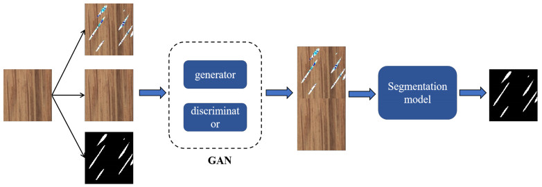
Anomaly detection is a binary classification task, which is to determine whether each pixel is abnormal or not. The difficulties are that it is hard to obtain abnormal samples and predict the shape of abnormal regions. Due to these difficulties, traditional supervised segmentation methods fail. The usual weakly supervised segmentation methods will use artificially generate defects to construct training samples. However, the model will be overfitted to artificially generated defects during training, resulting in insufficient generalization ability of the model. In this paper, we presented a novel reconstruction-based weakly supervised method for sparse anomaly detection. We proposed to use generative adversarial networks (GAN) to learn the distribution of positive samples, and reconstructed negative samples which contained the sparse defect into positive ones. Due to the nature of GAN, the training dataset only needs to contain normal samples. Subsequently, the segmentation network performs progressive feature fusion on reconstructed and original samples to complete the anomaly detection. Specifically, we designed the loss function based on kullback-leibler divergence for sparse anomalous defects. The final weakly-supervised segmentation network only assumes a sparsity prior of the defect region; thus, it can circumvent the detailed semantic labels and alleviate the potential overfitting problem. We compared our method with the state of the art generation-based generative anomaly detection methods and observed the average area under the receiver operating characteristic curve increase of 3% on MVTec anomaly detection.

| [1] | W. Samek, G. Montavon, S. Lapuschkin, C. J. Anders, K. Müller, Explaining deep neural networks and beyond: A review of methods and applications, in Proceedings of the IEEE, 109 (2021), 247–278. https://doi.org/10.1109/JPROC.2021.3060483 |
| [2] |
G. Quellec, M. Lamard, M. Cozic, G. Coatrieux, G. Cazuguel, Multiple-instance learning for anomaly detection in digital mammography, IEEE Trans. Med. Imaging, 35 (2016), 1604–1614. https://doi.org/10.1109/TMI.2016.2521442 doi: 10.1109/TMI.2016.2521442

|
| [3] |
S. Zhang, J. Li, L. Yang, Survey on low-level controllable image synthesis with deep learning, Electron. Res. Arch., 31 (2023), 7385–7426. https://doi.org/10.3934/era.2023374 doi: 10.3934/era.2023374
|
| [4] | S. Venkataramanan, K. Peng, R. V. Singh, A. Mahalanobis, Attention guided anomaly localization in images, in Computer Vision – ECCV 2020, 12362 (2020), 485–503. https://doi.org/10.1007/978-3-030-58520-4_29 |
| [5] |
T. Schlegl, P. Seeböck, S. M. Waldstein, G. Langs, U. Schmidt-Erfurth, f-AnoGAN: Fast unsupervised anomaly detection with generative adversarial networks, Med. Image Anal., 54 (2019), 30–44, https://doi.org/10.1016/j.media.2019.01.010 doi: 10.1016/j.media.2019.01.010
|
| [6] | L. Chen, G. Papandreou, F. Schroff, H. Adam, Rethinking atrous convolution for semantic image segmentation, preprint, arXiv: 1706.05587. |
| [7] | E. Bingham, H. Mannila, Random projection in dimensionality reduction: Applications to image and text data, in Proceedings of the seventh ACM SIGKDD international conference on Knowledge discovery and data mining, (2001), 245–250, https://doi.org/10.1145/502512.502546 |
| [8] |
T. Tang, W. Kuo, J. Lan, C. Ding, H. Hsu, H. Young, Anomaly detection neural network with dual auto-encoders gan and its industrial inspection applications, Sensors, 20 (2022), 3336. https://doi.org/10.3390/s20123336 doi: 10.3390/s20123336
|
| [9] | I. J. Goodfellow, J. Pouget-Abadie, M. Mirza, B. Xu, D. Warde-Farley, S. Ozair, et al., Generative adversarial networks, preprint, arXiv: 1406.2661. |
| [10] | S. Akcay, A. Atapour-Abarghouei, T. P. Breckon, GANomaly: Semi-supervised anomaly detection via adversarial training, in Computer Vision-ACCV 2018, 11363 (2018), 622–637. https://doi.org/10.1007/978-3-030-20893-6_39 |
| [11] | S. Akçay, A. Atapour-Abarghouei, T. P. Breckon, Skip-GANomaly: Skip connected and adversarially trained encoder-decoder anomaly detection, in 2019 International Joint Conference on Neural Networks (IJCNN), (2019), 1–8. https://doi.org/10.1109/IJCNN.2019.8851808 |
| [12] | U. Sivanesan, L. H. Braga, R. R. Sonnadara, K. Dhindsa, TricycleGAN: Unsupervised image synthesis and segmentation based on shape priors, preprint, arXiv: 2102.02690. |
| [13] |
V. Zavrtanik, M. Kristan, D. Skočaj, Reconstruction by inpainting for visual anomaly detection, Pattern Recognit., 112 (2021), 107706. https://doi.org/10.1016/j.patcog.2020.107706 doi: 10.1016/j.patcog.2020.107706
|
| [14] | M. Salehi, N. Sadjadi, S. Baselizadeh, M. H. Rohban, H. R. Rabiee, Multiresolution knowledge distillation for anomaly detection, in 2021 IEEE/CVF Conference on Computer Vision and Pattern Recognition (CVPR), (2021), 14897–14907. https://doi.org/10.1109/CVPR46437.2021.01466 |
| [15] | H. Deng, X. Li, Anomaly detection via reverse distillation from one-class embedding, in 2022 IEEE/CVF Conference on Computer Vision and Pattern Recognition (CVPR), (2022), 9727–9736. https://doi.org/10.1109/CVPR52688.2022.00951 |
| [16] | X. Zhang, M. Xu, X. Zhou, RealNet: A feature selection network with realistic synthetic anomaly for anomaly detection, preprint, arXiv: 2403.05897. |
| [17] |
E. Shelhamer, J. Long, T. Darrell, Fully convolutional networks for semantic segmentation, IEEE Trans. Pattern Anal. Mach. Intell., 39 (2017), 640–651. https://doi.org/10.1109/TPAMI.2016.2572683 doi: 10.1109/TPAMI.2016.2572683
|
| [18] | T. Lin, P. Dollár, R. Girshick, K. He, B. Hariharan, S. Belongie, Feature pyramid networks for object detection, in 2017 IEEE Conference on Computer Vision and Pattern Recognition (CVPR), (2017), 936–944. https://doi.org/10.1109/CVPR.2017.106 |
| [19] | O. Ronneberger, P. Fischer, T. Brox, U-Net: Convolutional networks for biomedical image segmentation, in Medical Image Computing and Computer-Assisted Intervention-MICCAI 2015, 9351 (2015), 234–241. https://doi.org/10.1007/978-3-319-24574-4_28 |
| [20] | K. Perlin, An image synthesizer, ACM SIGGRAPH Comput. Graphics, 19 (1985), 287–296, https://doi.org/10.1145/325165.325247 |
| [21] | D. P. Kingma, M. Welling, Auto-encoding variational bayes, preprint, arXiv: 1312.6114. |
| [22] |
Z. Wang, A. C. Bovik, H. R. Sheikh, E. P. Simoncelli, Image quality assessment: from error visibility to structural similarity, IEEE Trans. Image Process., 13 (2004), 600–612. https://doi.org/10.1109/TIP.2003.819861 doi: 10.1109/TIP.2003.819861
|
| [23] | K. He, X. Zhang, S. Ren, J. Sun, Deep residual learning for image recognition, in 2016 IEEE Conference on Computer Vision and Pattern Recognition (CVPR), (2016), 770–778. https://doi.org/10.1109/CVPR.2016.90 |
| [24] | T. Lin, P. Goyal, R. Girshick, K. He, P. Dollár, Focal loss for dense object detection, in 2017 IEEE International Conference on Computer Vision (ICCV), (2017), 2999–3007. https://doi.org/10.1109/ICCV.2017.324 |
| [25] |
O. Cappé, A. Garivier, O. Maillard, R. Munos, G. Stoltz, Kullback-Leibler upper confidence bounds for optimal sequential allocation, Ann. Stat., 41 (2013), 1516–1541, http://doi.org/10.1214/13-AOS1119 doi: 10.1214/13-AOS1119
|
| [26] | P. Bergmann, M. Fauser, D. Sattlegger, C. Steger, MVTec AD-A comprehensive real-world dataset for unsupervised anomaly detection, in 2019 IEEE/CVF Conference on Computer Vision and Pattern Recognition (CVPR), (2019), 9584–9592. https://doi.org/10.1109/CVPR.2019.00982 |
| [27] | P. Bergmann, M. Fauser, D. Sattlegger, C. Steger, Uninformed students: Student-teacher anomaly detection with discriminative latent embeddings, in 2020 IEEE/CVF Conference on Computer Vision and Pattern Recognition (CVPR), (2020), 4182–4191. https://doi.org/10.1109/CVPR42600.2020.00424 |
| [28] | D. Dehaene, O. Frigo, S. Combrexelle, P. Eline, Iterative energy-based projection on a normal data manifold for anomaly localization, preprint, arXiv: 2002.03734. |
| [29] | K. Zhou, Y. Xiao, J. Yang, J. Cheng, W. Liu, W. Luo, et al., Encoding structure-texture relation with P-Net for anomaly detection in retinal images, in Computer Vision-ECCV 2020, 12365 (2020), 360–377. https://doi.org/10.1007/978-3-030-58565-5_22 |


Figures(7) / Tables(4)
Kaixuan Wang, Shixiong Zhang, Yang Cao, Lu Yang. Weakly supervised anomaly detection based on sparsity prior[J]. Electronic Research Archive, 2024, 32(6): 3728-3741. doi: 10.3934/era.2024169


 DownLoad: