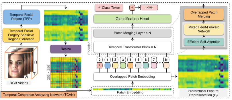
Current facial image manipulation techniques have caused public concerns while achieving impressive quality. However, these techniques are mostly bound to a single frame for synthesized videos and pay little attention to the most discriminatory temporal frequency artifacts between various frames. Detecting deepfake videos using temporal modeling still poses a challenge. To address this issue, we present a novel deepfake video detection framework in this paper that consists of two levels: temporal modeling and coherence analysis. At the first level, to fully capture temporal coherence over the entire video, we devise an efficient temporal facial pattern (TFP) mechanism that explores the color variations of forgery-sensitive facial areas by providing global and local-successive temporal views. The second level presents a temporal coherence analyzing network (TCAN), which consists of novel global temporal self-attention characteristics, high-resolution fine and low-resolution coarse feature extraction, and aggregation mechanisms, with the aims of long-range relationship modeling from a local-successive temporal perspective within a TFP and capturing the vital dynamic incoherence for robust detection. Thorough experiments on large-scale datasets, including FaceForensics++, DeepFakeDetection, DeepFake Detection Challenge, CelebDF-V2, and DeeperForensics, reveal that our paradigm surpasses current approaches and stays effective when detecting unseen sorts of deepfake videos.
Citation: Muhammad Ahmad Amin, Yongjian Hu, Jiankun Hu. Analyzing temporal coherence for deepfake video detection[J]. Electronic Research Archive, 2024, 32(4): 2621-2641. doi: 10.3934/era.2024119
Current facial image manipulation techniques have caused public concerns while achieving impressive quality. However, these techniques are mostly bound to a single frame for synthesized videos and pay little attention to the most discriminatory temporal frequency artifacts between various frames. Detecting deepfake videos using temporal modeling still poses a challenge. To address this issue, we present a novel deepfake video detection framework in this paper that consists of two levels: temporal modeling and coherence analysis. At the first level, to fully capture temporal coherence over the entire video, we devise an efficient temporal facial pattern (TFP) mechanism that explores the color variations of forgery-sensitive facial areas by providing global and local-successive temporal views. The second level presents a temporal coherence analyzing network (TCAN), which consists of novel global temporal self-attention characteristics, high-resolution fine and low-resolution coarse feature extraction, and aggregation mechanisms, with the aims of long-range relationship modeling from a local-successive temporal perspective within a TFP and capturing the vital dynamic incoherence for robust detection. Thorough experiments on large-scale datasets, including FaceForensics++, DeepFakeDetection, DeepFake Detection Challenge, CelebDF-V2, and DeeperForensics, reveal that our paradigm surpasses current approaches and stays effective when detecting unseen sorts of deepfake videos.

| [1] | M. Kowalski, Deepfakes. Available from: https://www.github.com/MarekKowalski/FaceSwap/. |
| [2] |
K. Liu, I. Perov, D. Gao, N. Chervoniy, W. Zhou, W. Zhang, Deepfacelab: integrated, flexible and extensible face-swapping framework, Pattern Recognit., 141 (2023), 109628. https://doi.org/10.1016/j.patcog.2023.109628 doi: 10.1016/j.patcog.2023.109628

|
| [3] | D. Afchar, V. Nozick, J. Yamagishi, I. Echizen, MesoNet: a compact facial video forgery detection network, in 2018 IEEE International Workshop on Information Forensics and Security (WIFS), (2018), 1–7. https://doi.org/10.1109/WIFS.2018.8630761 |
| [4] | F. Matern, C. Riess, M. Stamminger, Exploiting visual artifacts to expose deepfakes and face manipulations, in 2019 IEEE Winter Applications of Computer Vision Workshops (WACVW), (2019), 83–92. https://doi.org/10.1109/WACVW.2019.00020 |
| [5] | Y. Qian, G. Yin, L. Sheng, Z. Chen, J. Shao, Thinking in frequency: face forgery detection by mining frequency-aware clues, in ECCV 2020: Computer Vision – ECCV 2020, Springer-Verlag, (2020), 86–103. https://doi.org/10.1007/978-3-030-58610-2_6 |
| [6] | H. Liu, X. Li, W. Zhou, Y. Chen, Y. He, H. Xue, et al., Spatial-phase shallow learning: rethinking face forgery detection in bfrequency domain, in Proceedings of the IEEE/CVF Conference on Computer Vision and Pattern Recognition (CVPR), (2021), 772–781. |
| [7] | S. Chen, T. Yao, Y. Chen, S. Ding, J. Li, R. Ji, Local relation learning for face forgery detection, in Proceedings of the AAAI Conference on Artificial Intelligence, 35 (2021), 1081–1088. https://doi.org/10.1609/aaai.v35i2.16193 |
| [8] | Q. Gu, S. Chen, T. Yao, Y. Chen, S. Ding, R. Yi, Exploiting fine-grained face forgery clues via progressive enhancement learning, in Proceedings of the AAAI Conference on Artificial Intelligence, 36 (2022), 735–743. https://doi.org/10.1609/aaai.v36i1.19954 |
| [9] | X. Li, Y. Lang, Y. Chen, X. Mao, Y. He, S. Wang, et al., Sharp multiple instance learning for DeepFake video detection, in Proceedings of the 28th ACM International Conference on Multimedia, (2020), 1864–1872. https://doi.org/10.1145/3394171.3414034 |
| [10] | Z. Gu, Y. Chen, T. Yao, S. Ding, J. Li, F. Huang, et al., Spatiotemporal inconsistency learning for DeepFake video detection, in Proceedings of the 29th ACM International Conference on Multimedia, (2021), 3473–3481. https://doi.org/10.1145/3474085.3475508 |
| [11] | S. A. Khan, H. Dai, Video transformer for deepfake detection with incremental learning, in Proceedings of the 29th ACM International Conference on Multimedia, (2021), 1821–1828. http://doi.org/10.1145/3474085.3475332 |
| [12] | D. H. Choi, H. J. Lee, S. Lee, J. U. Kim, Y. M. Ro, Fake video detection with certainty-based attention network, in 2020 IEEE International Conference on Image Processing (ICIP), (2020), 823–827. http://doi.org/10.1109/ICIP40778.2020.9190655 |
| [13] | E. Sabir, J. Cheng, A. Jaiswal, W. Abdalmageed, I. Masi, P. Natarajan, Recurrent convolutional strategies for face manipulation detection in videos, Interfaces (GUI), (2019), 80–87. |
| [14] |
A. Chintha, B. Thai, S. J. Sohrawardi, K. Bhatt, A. Hickerson, M. Wright, et al., Recurrent convolutional structures for audio spoof and video deepfake detection, IEEE J. Sel. Top. Signal Process., 14 (2020), 1024–1037. http://doi.org/10.1109/JSTSP.2020.2999185 doi: 10.1109/JSTSP.2020.2999185
|
| [15] | A. Haliassos, K. Vougioukas, S. Petridis, M. Pantic, Lips don't lie: a generalisable and robust approach to face forgery detection, in Proceedings of the IEEE/CVF Conference on Computer Vision and Pattern Recognition (CVPR), (2021), 5039–5049. |
| [16] | Y. Zheng, J. Bao, D. Chen, M. Zeng, F. Wen, Exploring temporal coherence for more general video face forgery detection, in Proceedings of the IEEE/CVF International Conference on Computer Vision (ICCV), (2021), 15044–15054. |
| [17] | Z. Gu, Y. Chen, T. Yao, S. Ding, J. Li, L. Ma, Delving into the local: dynamic inconsistency learning for DeepFake video detection, in Proceedings of the AAAI Conference on Artificial Intelligence, 36 (2022), 744–752. http://doi.org/10.1609/aaai.v36i1.19955 |
| [18] | X. Zhao, Y. Yu, R. Ni, Y. Zhao, Exploring complementarity of global and local spatiotemporal information for fake face video detection, in ICASSP 2022 - 2022 IEEE International Conference on Acoustics, Speech and Signal Processing (ICASSP), (2022), 2884–2888. http://doi.org/10.1109/ICASSP43922.2022.9746061 |
| [19] | R. Shao, T. Wu, Z. Liu, Detecting and recovering sequential DeepFake manipulation, in ECCV 2022: Computer Vision – ECCV 2022, Springer-Verlag, (2022), 712–728. http://doi.org/10.1007/978-3-031-19778-9_41 |
| [20] | A. Dosovitskiy, L. Beyer, A. Kolesnikov, D. Weissenborn, X. Zhai, T. Unterthiner, et al., An image is worth 16 x 16 words: transformers for image recognition at scale, preprint, arXiv: 2010.11929. |
| [21] | A. Arnab, M. Dehghani, G. Heigold, C. Sun, M. Lučić, C. Schmid, ViViT: a video vision transformer, in Proceedings of the IEEE/CVF International Conference on Computer Vision (ICCV), (2021), 6836–6846. |
| [22] | Y. Zhang, X. Li, C. Liu, B. Shuai, Y. Zhu, B. Brattoli, et al., VidTr: Video transformer without convolutions, in Proceedings of the IEEE/CVF International Conference on Computer Vision (ICCV), (2021), 13577–13587. |
| [23] | L. He, Q. Zhou, X. Li, L. Niu, G. Cheng, X. Li, et al., End-to-end video object detection with spatial-temporal transformers, in Proceedings of the 29th ACM International Conference on Multimedia, (2021), 1507–1516. http://doi.org/10.1145/3474085.3475285 |
| [24] |
Z. Xu, D. Chen, K. Wei, C. Deng, H. Xue, HiSA: Hierarchically semantic associating for video temporal grounding, IEEE Trans. Image Process., 31 (2022), 5178–5188. http://doi.org/10.1109/TIP.2022.3191841 doi: 10.1109/TIP.2022.3191841
|
| [25] | O. de Lima, S. Franklin, S. Basu, B. Karwoski, A. George, Deepfake detection using spatiotemporal convolutional networks, preprint, arXiv: 2006.14749. |
| [26] | D. Güera, E. J. Delp, Deepfake video detection using recurrent neural networks, in 2018 15th IEEE International Conference on Advanced Video and Signal Based Surveillance (AVSS), (2018), 1–6. http://doi.org/10.1109/AVSS.2018.8639163 |
| [27] | I. Masi, A. Killekar, R. M. Mascarenhas, S. P. Gurudatt, W. AbdAlmageed, Two-branch recurrent network for isolating deepfakes in videos, in ECCV 2020: Computer Vision – ECCV 2020, Springer-Verlag, (2020), 667–684. http://doi.org/10.1007/978-3-030-58571-6_39 |
| [28] |
Y. Yu, R. Ni, Y. Zhao, S. Yang, F. Xia, N. Jiang, et al., MSVT: Multiple spatiotemporal views transformer for DeepFake video detection, IEEE Trans. Circuits Syst. Video Technol., 33 (2023), 4462–4471. http://doi.org/10.1109/TCSVT.2023.3281448 doi: 10.1109/TCSVT.2023.3281448
|
| [29] |
H. Cheng, Y. Guo, T. Wang, Q. Li, X. Chang, L. Nie, Voice-face homogeneity tells deepfake, ACM Trans. Multimedia Comput. Commun. Appl., 20 (2023), 1–22. http://doi.org/10.1145/3625231 doi: 10.1145/3625231
|
| [30] |
W. Yang, X. Zhou, Z. Chen, B. Guo, Z. Ba, Z. Xia, et al., AVoiD-DF: Audio-visual joint learning for detecting deepfake, IEEE Trans. Inf. Forensics Secur., 18 (2023), 2015–2029. http://doi.org/10.1109/TIFS.2023.3262148 doi: 10.1109/TIFS.2023.3262148
|
| [31] | M. Liu, J. Wang, X. Qian, H. Li, Audio-visual temporal forgery detection using embedding-level fusion and multi-dimensional contrastive loss, IEEE Trans. Circuits Syst. Video Technol., 2023. http://doi.org/10.1109/TCSVT.2023.3326694 |
| [32] |
Q. Yin, W. Lu, B. Li, J. Huang, Dynamic difference learning with spatio–temporal correlation for deepfake video detection, IEEE Trans. Inf. Forensics Secur., 18 (2023), 4046–4058. http://doi.org/10.1109/TIFS.2023.3290752 doi: 10.1109/TIFS.2023.3290752
|
| [33] |
Y. Wang, C. Peng, D. Liu, N. Wang, X. Gao, Spatial-temporal frequency forgery clue for video forgery detection in VIS and NIR scenario, IEEE Trans. Circuits Syst. Video Technol., 33 (2023), 7943–7956. http://doi.org/10.1109/TCSVT.2023.3281475 doi: 10.1109/TCSVT.2023.3281475
|
| [34] | D. E. King, Dlib-ml: A machine learning toolkit, J. Mach. Learn. Res., 10 (2009), 1755–1758. Available from: http://www.jmlr.org/papers/volume10/king09a/king09a.pdf. |
| [35] | A. Rossler, D. Cozzolino, L. Verdoliva, C. Riess, J. Thies, M. Niessner, FaceForensics++: Learning to detect manipulated facial images, in 2019 IEEE/CVF International Conference on Computer Vision (ICCV), (2019), 1–11. http://doi.org/10.1109/ICCV.2019.00009 |
| [36] | E. Xie, W. Wang, Z. Yu, A. Anandkumar, J. M. Alvarez, P. Luo, SegFormer: Simple and efficient design for semantic segmentation with transformers, in Advances in Neural Information Processing Systems, 34 (2021), 12077–12090. |
| [37] | W. Wang, E. Xie, X. Li, D. P. Fan, K. Song, D. Liang, et al., Pyramid vision transformer: a versatile backbone for dense prediction without convolutions, in Proceedings of the IEEE/CVF International Conference on Computer Vision (ICCV), (2021), 568–578. |
| [38] | X. Chu, Z. Tian, B. Zhang, X. Wan, C. Shen, Conditional positional encodings for vision transformers, preprint, arXiv: 2102.10882. |
| [39] | M. A. Islam, S. Jia, N. D. B. Bruce, How much position information do convolutional neural networks encode? preprint, arXiv: 2001.08248. |
| [40] | N. Dufour, A. Gully, P. Karlsson, A. V. Vorbyov, T. Leung, J. Childs, et al., Contributing data to Deepfake detection research by Google Research & Jigsaw, 2019. Available from: http://blog.research.google/2019/09/contributing-data-to-deepfake-detection.html. |
| [41] | B. Dolhansky, J. Bitton, B. Pflaum, J. Lu, R. Howes, M. Wang, et al., The DeepFake detection challenge (DFDC) dataset, preprint, arXiv: 2006.07397. |
| [42] | Y. Li, X. Yang, P. Sun, H. Qi, S. Lyu, Celeb-DF: A large-scale challenging dataset for DeepFake forensics, in Proceedings of the IEEE/CVF Conference on Computer Vision and Pattern Recognition (CVPR), (2020), 3207–3216. |
| [43] | L. Jiang, R. Li, W. Wu, C. Qian, C. C. Loy, DeeperForensics-1.0: A large-scale dataset for real-world face forgery detection, in Proceedings of the IEEE/CVF Conference on Computer Vision and Pattern Recognition (CVPR), (2020), 2889–2898. |
| [44] |
A. P. Bradley, The use of the area under the ROC curve in the evaluation of machine learning algorithms, Pattern Recognit., 30 (1997), 1145–1159. http://doi.org/10.1016/S0031-3203(96)00142-2 doi: 10.1016/S0031-3203(96)00142-2
|
| [45] | P. Micikevicius, S. Narang, J. Alben, G. F. Diamos, E. Elsen, D. Garcia, et al., Mixed precision training, preprint, arXiv: 1710.03740. |
| [46] | Z. Zhang, M. R. Sabuncu, Generalized cross entropy loss for training deep neural networks with noisy labels, in Advances in Neural Information Processing Systems, 31 (2018). |
| [47] | L. van der Maaten, G. Hinton, Visualizing data using t-SNE, J. Mach. Learn. Res., 9 (2008), 2579–2605. |
| [48] | I. Radosavovic, R. P. Kosaraju, R. Girshick, K. He, P. Dollár, Designing network design spaces, in 2020 IEEE/CVF Conference on Computer Vision and Pattern Recognition (CVPR), (2020), 10425–10433. http://doi.org/10.1109/CVPR42600.2020.01044 |
| [49] | Z. Liu, H. Hu, Y. Lin, Z. Yao, Z. Xie, Y. Wei, et al., Swin transformer v2: Scaling up capacity and resolution, in Proceedings of the IEEE/CVF Conference on Computer Vision and Pattern Recognition (CVPR), (2022), 12009–12019. |
| [50] | H. Bao, L. Dong, S. Piao, F. Wei, BEiT: BERT pre-training of image transformers, preprint, arXiv: 2106.08254. |
| [51] | W. Yu, M. Luo, P. Zhou, C. Si, Y. Zhou, X. Wang, et al., Metaformer is actually what you need for vision, in Proceedings of the IEEE/CVF Conference on Computer Vision and Pattern Recognition (CVPR), (2022), 10819–10829. |


Figures(6) / Tables(6)
Muhammad Ahmad Amin, Yongjian Hu, Jiankun Hu. Analyzing temporal coherence for deepfake video detection[J]. Electronic Research Archive, 2024, 32(4): 2621-2641. doi: 10.3934/era.2024119


 DownLoad: