Spatiotemporal variation of the major meteorological elements in an agricultural region: A case study of Linyi City, Northern China

Li Li; Xiaoning Lu; Wu Jun; Li Li; Xiaoning Lu; Wu Jun

doi:10.3934/era.2024112

Electronic Research Archive

2024, Volume 32, Issue 4: 2447-2465. doi: 10.3934/era.2024112

Previous Article Next Article

Research article

Spatiotemporal variation of the major meteorological elements in an agricultural region: A case study of Linyi City, Northern China

1.
Linyi Meteorological Bureau of Shandong Province, Linyi 276000, China
2.
Faculty of Environment and Life, Beijing University of Technology, Beijing 100124, China
3.
Shandong Provincial Key Laboratory of Meteorological Disaster Prevention and Mitigation, Jinan 250000, China
4.
College of Resources and Environment, Chengdu University of Information Technology, Chengdu 610000, China
Correction on: Electronic Research Archive 32: 3313-3315.

Received: 24 September 2023 Revised: 08 March 2024 Accepted: 11 March 2024 Published: 26 March 2024

Evaporation is a key element of the water and energy cycle and is essential in determining the spatial and temporal variations of meteorological elements. In particular, evaporation is crucial for thoroughly understanding the climate variations of a region. In this study, we discussed evaporation, precipitation, and temperature by adopting Linyi City in Shandong Province, China, which is an important agricultural region, as a research case. Linear regression analysis, the empirical orthogonal decomposition function, and the Morlet wavelet function were used to reveal the trends, spatiotemporal modes, and multi-time scale characteristics of the three climate factors and provide a theoretical basis for the efficient use of climate resources in the future development of regional agriculture. Results showed that the precipitation (2.09 mm/a) and temperature (0.04 ℃/a) in Linyi City exhibited a synchronous growth trend. Conversely, evaporation (−6.47 mm/a) showed a decreasing trend and the evaporation paradox because of the considerable decrease in evaporation energy. Regional development of water-consuming agriculture in consideration of global warming is a key point for improving water use efficiency in Linyi City. In terms of spatial distribution, precipitation was dominated by the first mode wherein low precipitation was observed at the early stage, and high precipitation occurred at the late stage. The first mode was supplemented by the second mode wherein an inverse phase change occurred in the southeast-northwest direction. Large interannual fluctuations were observed only in Yinan County. Temperature exhibited a pattern of warming change with high homogeneity. Evaporation demonstrated obvious heterogeneity and was dominated by two major modes, and the difference in evaporation between Junan County and the other regions of Linyi City was large. Therefore, the local regional climate changes in Yinan and Junan should be given attention. All three meteorological elements showed interannual and interdecadal variations in the short (5 a), medium (16 a), and long (25 a) terms, with precipitation, temperature, and evaporation dominated by 16 a, 24 a, and 31 a, respectively. In the short-term future, the regional precipitation and temperature in Linyi will experience decrements that are above the multiyear average, and evaporation will increase to above the multiyear average. Given the changing trends of precipitation, temperature, and evaporation, urgent requirements for the regional development of efficient water-saving irrigation and the promotion of digital agriculture should be proposed.
- precipitation,
- temperature,
- evaporation,
- Linyi,
- spatiotemporal variation
Citation: Li Li, Xiaoning Lu, Wu Jun. Spatiotemporal variation of the major meteorological elements in an agricultural region: A case study of Linyi City, Northern China[J]. Electronic Research Archive, 2024, 32(4): 2447-2465. doi: 10.3934/era.2024112

Related Papers:

Abstract

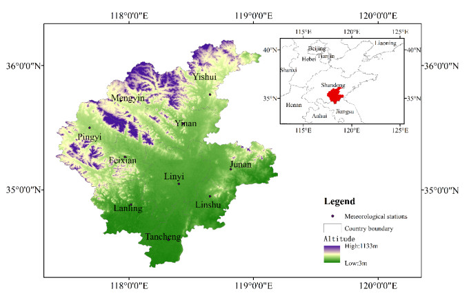
Evaporation is a key element of the water and energy cycle and is essential in determining the spatial and temporal variations of meteorological elements. In particular, evaporation is crucial for thoroughly understanding the climate variations of a region. In this study, we discussed evaporation, precipitation, and temperature by adopting Linyi City in Shandong Province, China, which is an important agricultural region, as a research case. Linear regression analysis, the empirical orthogonal decomposition function, and the Morlet wavelet function were used to reveal the trends, spatiotemporal modes, and multi-time scale characteristics of the three climate factors and provide a theoretical basis for the efficient use of climate resources in the future development of regional agriculture. Results showed that the precipitation (2.09 mm/a) and temperature (0.04 ℃/a) in Linyi City exhibited a synchronous growth trend. Conversely, evaporation (−6.47 mm/a) showed a decreasing trend and the evaporation paradox because of the considerable decrease in evaporation energy. Regional development of water-consuming agriculture in consideration of global warming is a key point for improving water use efficiency in Linyi City. In terms of spatial distribution, precipitation was dominated by the first mode wherein low precipitation was observed at the early stage, and high precipitation occurred at the late stage. The first mode was supplemented by the second mode wherein an inverse phase change occurred in the southeast-northwest direction. Large interannual fluctuations were observed only in Yinan County. Temperature exhibited a pattern of warming change with high homogeneity. Evaporation demonstrated obvious heterogeneity and was dominated by two major modes, and the difference in evaporation between Junan County and the other regions of Linyi City was large. Therefore, the local regional climate changes in Yinan and Junan should be given attention. All three meteorological elements showed interannual and interdecadal variations in the short (5 a), medium (16 a), and long (25 a) terms, with precipitation, temperature, and evaporation dominated by 16 a, 24 a, and 31 a, respectively. In the short-term future, the regional precipitation and temperature in Linyi will experience decrements that are above the multiyear average, and evaporation will increase to above the multiyear average. Given the changing trends of precipitation, temperature, and evaporation, urgent requirements for the regional development of efficient water-saving irrigation and the promotion of digital agriculture should be proposed.

References

[1]	Y. Wang, A. Wang, J. Zhai, H. Tao, T. Jiang, B. Su, et al., Tens of thousands additional deaths annually in cities of China between 1.5 ℃ and 2.0 ℃ warming, Nat. Commun., 10 (2019), 3376. https://doi.org/10.1038/s41467-019-11283-w doi: 10.1038/s41467-019-11283-w
[2]	Z. Zhou, Y. Ding, H. Shi, H. Cai, Q. Fu, S. Liu, et al., Analysis and prediction of vegetation dynamic changes in China: Past, present and future, Ecol. Indic., 117 (2020), 106642. https://doi.org/10.1016/j.ecolind.2020.106642 doi: 10.1016/j.ecolind.2020.106642
[3]	W. Yang, L. Zhang, Z. Yang, Spatiotemporal characteristics of droughts and floods in Shandong Province, China and their relationship with food loss, Chin. Geogr. Sci., 33 (2023), 304–319. https://doi.org/10.1007/s11769-023-1338-0 doi: 10.1007/s11769-023-1338-0
[4]	Y. Tang, W. Cai, J. Zhai, S. Wang, Y. Liu, Y. Chen, et al., Climatic anomalous features and major meteorological disasters in China in summer of 2021 (in Chinese), Arid Meteorol., 40 (2022), 179–186.
[5]	Z. Shu, W. Li, J. Zhang, J. Jin, Q. Xue, Y. Wang, et al., Historical changes and future trends of extreme precipitation and high temperature in China, Chin. J. Eng. Sci., 24 (2022), 116–125. https://doi.org/10.15302/j-sscae-2022.05.014 doi: 10.15302/j-sscae-2022.05.014
[6]	B. Li, X. Shi, L. Lian, Y. Chen, Z. Chen, X. Sun, Quantifying the effects of climate variability, direct and indirect land use change, and human activities on runoff, J. Hydrol., 584 (2020), 124684. https://doi.org/10.1016/j.jhydrol.2020.124684
[7]	Y. Liu, M. You, J. Zhu, F. Wang, R. Ran, Integrated risk assessment for agricultural drought and flood disasters based on entropy information diffusion theory in the middle and lower reaches of the Yangtze River, China, Int. J. Disaster Risk Reduct., 38 (2019), 101194. https://doi.org/10.1016/j.ijdrr.2019.101194
[8]	Y. Li, H. Li, D. Li, Z. Zhang, Y. Feng, Construction of rural water ecological civilization index system in China, Water Pract. Technol., 15 (2020), 797–806. https://doi.org/10.2166/wpt.2020.064 doi: 10.2166/wpt.2020.064
[9]	J. Ren, S. Gu, C. Feng, X. Lu, Analysis of spatial and temporal variability of temperature and precipitation in Shandong Province in the context of climate change (in Chinese), Water Resour. Hydropower Eng., 54 (2023), 27–37. https://doi.org/10.13928/j.cnki.wrahe.2023.05.003 doi: 10.13928/j.cnki.wrahe.2023.05.003
[10]	X. Dong, W. Gu, X. Meng, H. Liu, Characteristics of changes in precipitation events in Shandong Province in the past 50 years (in Chinese), Acta Geogr. Sin., 69 (2014), 661–671.
[11]	Z. Cheng, B. Lu, H. Wang, S. Xiong, Y. Hu, Analysis and prediction of climate elements change characteristics in Shandong region (in Chinese), Water Resour. Power, 35 (2017), 10–14.
[12]	W. Wu, X. Tang, N. Guo, C. Yang, H. Liu, Y. Shang, Spatiotemporal modeling of monthly soil temperature using artificial neural networks, Theor. Appl. Climatol., 113 (2013), 481–494. https://doi.org/10.1007/s00704-012-0807-7 doi: 10.1007/s00704-012-0807-7
[13]	L. Xu, P. Zhang, C. Wang, K. Wang, Wavelet analysis and trend prediction of temperature change in Linyi City (in Chinese), Agric. Technol., 38 (2018), 120–123.
[14]	R. Zhang, Y. Qu, X. Zhang, X. Wu, X. Zhou, B. Ren, et al., Spatiotemporal variability in annual drought severity, duration, and frequency from 1901 to 2020, Clim. Res., 87 (2022), 81–97. https://doi.org/10.3354/cr01680 doi: 10.3354/cr01680
[15]	A. K. Yetik, B. Arslan, B. Şen, Trends and variability in precipitation across Turkey: A multimethod statistical analysis, Theor. Appl. Climatol., 155 (2024), 473–488. https://doi.org/10.1007/s00704-023-04645-4 doi: 10.1007/s00704-023-04645-4
[16]	Y. Zhao, Y. Luo, Wavelet analysis on temperature and precipitation changes in Dabie Mountain of West Anhui, J. Phys. Conf. Ser., 1732 (2021), 012105. https://doi.org/10.1088/1742-6596/1732/1/012105 doi: 10.1088/1742-6596/1732/1/012105
[17]	B. Song, K. Park, Temperature trend analysis associated with land-cover changes using time-series data (1980–2019) from 38 weather stations in South Korea, Sustainable Cities Soc., 65 (2021), 102615. https://doi.org/10.1016/j.scs.2020.102615 doi: 10.1016/j.scs.2020.102615
[18]	G. Bürger, Intraseasonal oscillation indices from complex EOFs, J. Clim., 34 (2021), 107–122. https://doi.org/10.1175/jcli-d-20-0427.1 doi: 10.1175/jcli-d-20-0427.1
[19]	X. Chen, J. M. Wallace, K. K. Tung, Pairwise-rotated EOFs of global SST, J. Clim., 30 (2017), 5473–5489. https://doi.org/10.1175/jcli-d-16-0786.1 doi: 10.1175/jcli-d-16-0786.1
[20]	G. R. North, T. L. Bell, R. F. Cahalan, F. J. Moeng, Sampling errors in the estimation of empirical orthogonal functions, Mon. Weather Rev., 110 (1982), 699–706. https://doi.org/10.1175/1520-0493(1982)110<0699:seiteo>2.0.co;2 doi: 10.1175/1520-0493(1982)110<0699:seiteo>2.0.co;2
[21]	Q. Li, P. He, Y. He, X. Han, T. Zeng, G. Lu, et al., Investigation to the relation between meteorological drought and hydrological drought in the upper Shaying River Basin using wavelet analysis, Atmos. Res., 234 (2020), 104743. https://doi.org/10.1016/j.atmosres.2019.104743 doi: 10.1016/j.atmosres.2019.104743
[22]	V. Cheng, A. Saber, C. A. Arnillas, A. Javed, A. Richards, G. B. Arhonditsis, Effects of hydrological forcing on short- and long-term water level fluctuations in Lake Huron-Michigan: A continuous wavelet analysis. J. Hydrol., 603 (2021), 127164. https://doi.org/10.1016/j.jhydrol.2021.127164
[23]	E. Lee, S. Kim, Wavelet analysis of soil moisture measurements for hillslope hydrological processes, J. Hydrol., 575 (2019), 82–93. https://doi.org/10.1016/j.jhydrol.2019.05.023 doi: 10.1016/j.jhydrol.2019.05.023
[24]	H. Xu, B. Lei, Z. Li, A reconstruction of total solar irradiance based on wavelet analysis, Earth Space Sci., 8 (2021), e2021EA001819. https://doi.org/10.1029/2021ea001819 doi: 10.1029/2021ea001819
[25]	T. Guo, T. Zhang, E. Lim, M. Lopez-Benitez, F. Ma, L. Yu, A review of wavelet analysis and its applications: Challenges and opportunities, IEEE Access, 10 (2022), 58869–58903. https://doi.org/10.1109/ACCESS.2022.3179517 doi: 10.1109/ACCESS.2022.3179517
[26]	Z. Yan, S. Wang, D. Ma, B. Liu, H. Lin, S. Li, Meteorological factors affecting pan evaporation in the Haihe River Basin, China, Water, 11 (2019), 317. https://doi.org/10.3390/w11020317
[27]	T. Gao, X. Shi, Spatio-temporal characteristics of extreme precipitation events during 1951–2011 in Shandong, China and possible connection to the large scale atmospheric circulation, Stochastic Environ. Res. Risk Assess., 30 (2016), 1421–1440. https://doi.org/10.1007/s00477-015-1149-7
[28]	H. Li, S. Liu, M. Yin, L. Zhu, E. Shen, B. Sun, et al., Spatial and temporal variability and risk assessment of regional climate change in northern China: A case study in Shandong Province, Nat. Hazard., 111 (2022), 2749–2786. https://doi.org/10.1007/s11069-021-05156-z doi: 10.1007/s11069-021-05156-z
[29]	P. Sun, W. Qu, X. Zhu, Y. Wu, J. Wang, B. Zhang, et al., Variation of hydrothermal pattern of Huai River Basin from 1959 to 2018, (in Chinese), Resour. Environ. Yangtze Basin, 30 (2021), 1366–1377.
[30]	J. Hu, G. Zhao, P. Li, X. Mu, Variations of pan evaporation and its attribution from 1961 to 2015 on the Loess Plateau, China, Nat. Hazard., 111 (2022), 1199–1217. https://doi.org/10.1007/s11069-021-05091-z
[31]	Z. Liu, L. Zhangzhong, W. Zheng, X. Zhang, J. Yu, F. Zhang, et al., Analysis of the variation tendency and influencing factors of reference evapotranspiration in Shandong Province, China, Irrig. Drain., 72 (2023), 390–407. https://doi.org/10.1002/ird.2776 doi: 10.1002/ird.2776
[32]	M. Li, R. Chu, S. Shen, A. Islam, Quantifying climatic impact on reference evapotranspiration trends in the Huai River Basin of Eastern China, Water, 10 (2018), 144. https://doi.org/10.3390/w10020144 doi: 10.3390/w10020144
[33]	X. Huang, M. Liu, R. Chen, S. Gao, Q. Xie, Q. Feng, Evaluation and spatiotemporal characteristics of atmospheric environment efficiency in Shandong province based on super-SBM model, Environ. Res. Commun., 3 (2021), 115002. https://doi.org/10.1088/2515-7620/ac3409 doi: 10.1088/2515-7620/ac3409
[34]	X. Yan, A. Mohammadian, R. Ao, J. Liu, X. Chen, Spatiotemporal variations in reference evapotranspiration and its contributing climatic variables at various spatial scales across China for 1984–2019, Water, 14 (2022), 2502. https://doi.org/10.3390/w14162502 doi: 10.3390/w14162502
[35]	W. Ding, X. Zhao, K. Wang, Z. Xu, Y. Zhang, D. Wu, et al., Analysis on precipitation change characteristics in Linyi City from 1951 to 2016 (in Chinese), Mod. Agric. Sci. Technol., 10 (2018), 205–206+211.
[36]	J. A. J. Mendes, N. G. P. Carvalho, M. N. Mourarias, C. B. Careta, V. G. Zuin, M. C. Gerolamo, Dimensions of digital transformation in the context of modern agriculture, Sustain. Prod. Consum., 34 (2022), 613–637. https://doi.org/10.1016/j.spc.2022.09.027 doi: 10.1016/j.spc.2022.09.027

Reader Comments

Your name:*

Email:*
© 2024 the Author(s), licensee AIMS Press. This is an open access article distributed under the terms of the Creative Commons Attribution License (http://creativecommons.org/licenses/by/4.0)