Modeling the SARS-CoV-2 sublineages XBB and BQ.1 in Mexico, considering multiple vaccinations, booster dose, waning immunity and cross-immunity

Ugo Avila-Ponce de León; Angel G. C. Pérez; Eric Avila-Vales; Ugo Avila-Ponce de León; Angel G. C. Pérez; Eric Avila-Vales

doi:10.3934/era.2024053

Electronic Research Archive

2024, Volume 32, Issue 2: 1082-1125. doi: 10.3934/era.2024053

Previous Article Next Article

Research article

Modeling the SARS-CoV-2 sublineages XBB and BQ.1 in Mexico, considering multiple vaccinations, booster dose, waning immunity and cross-immunity

1.
Human Systems Biology Laboratory, Instituto Nacional de Medicina Genómica (INMEGEN), Mexico City, Mexico
2.
Facultad de Matemáticas, Universidad Autónoma de Yucatán, Anillo Periférico Norte, Tablaje Catastral 13615, C.P. 97119, Mérida, Yucatán, Mexico

Received: 09 October 2023 Revised: 24 November 2023 Accepted: 22 December 2023 Published: 25 January 2024

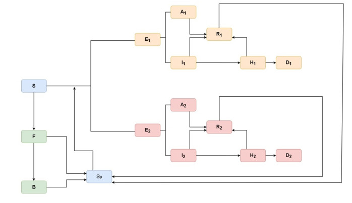
In a population with ongoing vaccinations, the trajectory of a pandemic is determined by how the virus spreads in the unvaccinated, vaccinated without boosters, and vaccinated with boosters, which will exhibit distinct transmission dynamics based on different levels of natural and vaccine-induced immunity. We found that enhancing the use of face masks in a partially vaccinated population is associated with a reduction of new infections, hospitalizations, and deaths. We highly recommend the use of a face mask with at least a 50% efficiency, such as improved cloth and surgical face masks, due to its effectivity and cost ratio. Our simulations indicated that there may be two upcoming Omicron waves (in the last months of 2022 and in May 2023). The magnitude of these waves will be 75% and 40% lower than their prior wave. Moreover, the size of these waves is heavily influenced by immunity parameters like waning immunity and cross-immunity protection. Hence, we recommend continuing the use of face masks to decrease transmission because we are not developing sterilizing immunity if we get infected by a prior sublineage, meaning that we can still get infected regardless of the acquired immunity.
- Omicron,
- vaccination,
- waning immunity,
- ordinary differential equations,
- Mexico,
- vaccine heterogeneity,
- COVID-19
Citation: Ugo Avila-Ponce de León, Angel G. C. Pérez, Eric Avila-Vales. Modeling the SARS-CoV-2 sublineages XBB and BQ.1 in Mexico, considering multiple vaccinations, booster dose, waning immunity and cross-immunity[J]. Electronic Research Archive, 2024, 32(2): 1082-1125. doi: 10.3934/era.2024053

Related Papers:

Abstract

In a population with ongoing vaccinations, the trajectory of a pandemic is determined by how the virus spreads in the unvaccinated, vaccinated without boosters, and vaccinated with boosters, which will exhibit distinct transmission dynamics based on different levels of natural and vaccine-induced immunity. We found that enhancing the use of face masks in a partially vaccinated population is associated with a reduction of new infections, hospitalizations, and deaths. We highly recommend the use of a face mask with at least a 50% efficiency, such as improved cloth and surgical face masks, due to its effectivity and cost ratio. Our simulations indicated that there may be two upcoming Omicron waves (in the last months of 2022 and in May 2023). The magnitude of these waves will be 75% and 40% lower than their prior wave. Moreover, the size of these waves is heavily influenced by immunity parameters like waning immunity and cross-immunity protection. Hence, we recommend continuing the use of face masks to decrease transmission because we are not developing sterilizing immunity if we get infected by a prior sublineage, meaning that we can still get infected regardless of the acquired immunity.

References

[1]	E. Dong, H. Du, L. Gardner, An interactive web-based dashboard to track COVID-19 in real time, Lancet Infect. Dis., 20 (2020), 533–534. https://doi.org/10.1016/S1473-3099(20)30120-1 doi: 10.1016/S1473-3099(20)30120-1
[2]	E. Mathieu, H. Ritchie, L. Rodés-Guirao, C. Appel, C. Giattino, J. Hasell, et al., Coronavirus pandemic (COVID-19), Our World in Data. Available from: https://ourworldindata.org/coronavirus.
[3]	Secretaría de Salud, Sana distancia COVID-19, Gobierno de México. Available from: https://www.gob.mx/salud/documentos/sana-distancia.
[4]	Gobierno de México, Semáforo COVID-19. Available from: https://web.archive.org/web/20220630213907/https://coronavirus.gob.mx/semaforo/.
[5]	Comisión Federal para la Protección contra Riesgos Sanitarios, Vacunas COVID 19 autorizadas, Gobierno de México. Available from: https://www.gob.mx/cofepris/acciones-y-programas/vacunas-covid-19-autorizadas.
[6]	L. Matrajt, J. Eaton, T. Leung, E. R. Brown, Vaccine optimization for COVID-19: Who to vaccinate first, Sci. Adv., 7 (2021), eabf1374. https://doi.org/10.1126/sciadv.abf1374 doi: 10.1126/sciadv.abf1374
[7]	K. M. Bubar, K. Reinholt, S. M. Kissler, M. Lipsitch, S. Cobey, Y. H. Grad, et al., Model-informed COVID-19 vaccine prioritization strategies by age and serostatus, Science, 371 (2021), 916–921. https://doi.org/10.1126/science.abe6959 doi: 10.1126/science.abe6959
[8]	Secretaría de Salud, Vacuna Covid–Sitio informativo. Available from: https://web.archive.org/web/20220808220248/http://vacunacovid.gob.mx/wordpress/.
[9]	M. M. Alvarez, S. Bravo-González, G. Trujillo-de Santiago, Modeling vaccination strategies in an Excel spreadsheet: Increasing the rate of vaccination is more effective than increasing the vaccination coverage for containing COVID-19, PLoS One, 16 (2021), e0254430. https://doi.org/10.1371/journal.pone.0254430 doi: 10.1371/journal.pone.0254430
[10]	A. del C. Munguía-López, J. M. Ponce-Ortega, Fair allocation of potential COVID-19 vaccines using an optimization-based strategy, Process Integr. Optim. Sustainability, 5 (2021), 3–12. https://doi.org/10.1007/s41660-020-00141-8 doi: 10.1007/s41660-020-00141-8
[11]	I. Soria-Arguello, R. Torres-Escobar, H. A. Pérez-Vicente, T. G. Perea-Rivera, A proposal mathematical model for the vaccine COVID-19 distribution network: A case study in Mexico, Math. Probl. Eng., 2021 (2021), 5484101. https://doi.org/10.1155/2021/5484101 doi: 10.1155/2021/5484101
[12]	F. Saldaña, J. X. Velasco-Hernández, The trade-off between mobility and vaccination for COVID-19 control: A metapopulation modelling approach, Royal Soc. Open Sci., 8 (2021), 202240. https://doi.org/10.1098/rsos.202240 doi: 10.1098/rsos.202240
[13]	A. S. Lauring, E. B. Hodcroft, Genetic variants of SARS-CoV-2—What do they mean, JAMA, 325 (2021), 529–531. https://doi.org/10.1001/jama.2020.27124 doi: 10.1001/jama.2020.27124
[14]	A. M. Gravagnuolo, L. Faqih, C. Cronshaw, J. Wynn, L. Burglin, P. Klapper, et al., Epidemiological investigation of new SARS-CoV-2 variant of concern 202012/01 in England, preprint, medRxiv: 2021.01.14.21249386.
[15]	S. Zárate, B. Taboada, J. E. Muñoz-Medina, P. Iša, A. Sanchez-Flores, C. Boukadida, et al., The Alpha variant (B.1.1.7) of SARS-CoV-2 failed to become dominant in Mexico, Microbiol. Spectrum, 10 (2022), e02240–21. https://doi.org/10.1128/spectrum.02240-21 doi: 10.1128/spectrum.02240-21
[16]	B. Taboada, S. Zárate, P. Iša, C. Boukadida, J. A. Vazquez-Perez, J. E. Muñoz-Medina, et al., Genetic analysis of SARS-CoV-2 variants in Mexico during the first year of the COVID-19 pandemic, Viruses, 13 (2021), 2161. https://doi.org/10.3390/v13112161 doi: 10.3390/v13112161
[17]	B. Taboada, S. Zárate, R. García-López, J. E. Muñoz-Medina, A. Sanchez-Flores, A. Herrera-Estrella, et al., Dominance of three sublineages of the SARS-CoV-2 Delta variant in Mexico, Viruses, 14 (2022), 1165. https://doi.org/10.3390/v14061165 doi: 10.3390/v14061165
[18]	S. Mallapaty, Where did Omicron come from? Three key theories, Nature, 602 (2022), 26–28. https://doi.org/10.1038/d41586-022-00215-2 doi: 10.1038/d41586-022-00215-2
[19]	R. Viana, S. Moyo, D. G. Amoako, H. Tegally, C. Scheepers, C. L. Althaus, et al., Rapid epidemic expansion of the SARS-CoV-2 Omicron variant in southern Africa, Nature, 603 (2022), 679–686. https://doi.org/10.1038/s41586-022-04411-y doi: 10.1038/s41586-022-04411-y
[20]	H. Gruell, K. Vanshylla, P. Tober-Lau, D. Hillus, P. Schommers, C. Lehmann, et al., mRNA booster immunization elicits potent neutralizing serum activity against the SARS-CoV-2 Omicron variant, Nat. Med., 28 (2022), 477–480. https://doi.org/10.1038/s41591-021-01676-0 doi: 10.1038/s41591-021-01676-0
[21]	K. Khan, F. Karim, Y. Ganga, M. Bernstein, Z. Jule, K. Reedoy, et al., Omicron sub-lineages BA.4/BA.5 escape neutralizing immunity elicited by BA.1 infection, Nat. Commun., 13 (2022), 4686. https://doi.org/10.1038/s41467-022-32396-9 doi: 10.1038/s41467-022-32396-9
[22]	Outbreak.info, SARS-CoV-2 (hCoV-19) mutation reports–lineage comparison, Enabled by data from GISAID. Available from: https://outbreak.info/compare-lineages?pango=BA.5&pango=BA.4&pango=BA.2.12.1&pango=BA.2&pango=BA.1&gene=ORF1a&gene=ORF1b&gene=S&gene=ORF3a&gene=E&gene=M&gene=ORF6&gene=ORF7a&gene=ORF7b&gene=ORF8&gene=N&gene=ORF10&threshold=75&nthresh=1&sub=false&dark=true.
[23]	H. N. Altarawneh, H. Chemaitelly, H. Ayoub, M. R. Hasan, P. Coyle, H. M. Yassine, et al., Protection of SARS-CoV-2 natural infection against reinfection with the BA.4 or BA.5 Omicron subvariants, preprint, medRxiv: 10.1101/2022.07.11.22277448.
[24]	MexCoV2, Consorcio Mexicano de Vigilancia Genómica, (CoViGen-Mex). Available from: http://mexcov2.ibt.unam.mx: 8080/COVID-TRACKER/.
[25]	Gobierno de México, Secretaría de Salud abre registro para vacuna de refuerzo a personas de 30 a 39 años, Secretaría de Salud. Available from: https://www.gob.mx/salud/prensa/056-secretaria-de-salud-abre-registro-para-vacuna-de-refuerzo-a-personas-de-30-a-39-anos.
[26]	L. Benahmadi, M. Lhous, A. Tridane, O. Zakary, M. Rachik, Modeling the impact of the imperfect vaccination of the COVID-19 with optimal containment strategy, Axioms, 11 (2022), 124. https://doi.org/10.3390/axioms11030124 doi: 10.3390/axioms11030124
[27]	C. J. Edholm, B. Levy, L. Spence, F. B. Agusto, F. Chirove, C. W. Chukwu, et al., A vaccination model for COVID-19 in Gauteng, South Africa, Infect. Dis. Modell., 7 (2022), 333–345. https://doi.org/10.1016/j.idm.2022.06.002 doi: 10.1016/j.idm.2022.06.002
[28]	G. G. Parra, A. J. Arenas, A nonlinear mathematical model for the dynamics of the Omicron wave, preprint, SSRN: 4119450. https://doi.org/10.2139/ssrn.4119450
[29]	S. Safdar, C. N. Ngonghala, A. Gumel, Mathematical assessment of the role of waning and boosting immunity against the BA.1 Omicron variant in the United States, Math. Biosci. Eng., 20 (2023), 179–212. https://doi.org/10.3934/mbe.2023009 doi: 10.3934/mbe.2023009
[30]	K. Koelle, M. A. Martin, R. Antia, B. Lopman, N. E. Dean, The changing epidemiology of SARS-CoV-2, Science, 375 (2022), 1116–1121. https://doi.org/10.1126/science.abm4915 doi: 10.1126/science.abm4915
[31]	A. G. C. Pérez, D. A. Oluyori, An extended SEIARD model for COVID-19 vaccination in Mexico: Analysis and forecast, Math. Appl. Sci. Eng., 2 (2021), 219–309. https://doi.org/10.5206/mase/14233 doi: 10.5206/mase/14233
[32]	F. J. Aguilar-Canto, U. Avila-Ponce de León, E. Avila-Vales, Sensitivity theorems of a model of multiple imperfect vaccines for COVID-19, Chaos Solitons Fractals, 156 (2022), 111844. https://doi.org/10.1016/j.chaos.2022.111844 doi: 10.1016/j.chaos.2022.111844
[33]	F. M. G. Magpantay, Vaccine impact in homogeneous and age-structured models, J. Math. Biol., 75 (2017), 1591–1617. https://doi.org/10.1007/s00285-017-1126-5 doi: 10.1007/s00285-017-1126-5
[34]	D. A. Swan, A. Goyal, C. Bracis, M. Moore, E. Krantz, E. Brown, et al., Mathematical modeling of vaccines that prevent SARS-CoV-2 transmission, Viruses, 13 (2021), 1921. https://doi.org/10.3390/v13101921 doi: 10.3390/v13101921
[35]	U. Avila-Ponce de León, E. Avila-Vales, K. L. Huang, Modeling COVID-19 dynamic using a two-strain model with vaccination, Chaos Solitons Fractals, 157 (2022), 111927. https://doi.org/10.1016/j.chaos.2022.111927 doi: 10.1016/j.chaos.2022.111927
[36]	Johns Hopkins CSSE, 2019 Novel Coronavirus COVID-19 (2019-nCoV) Data Repository. Available from: https://github.com/CSSEGISandData/COVID-19.
[37]	Institute for Health Metrics and Evaluation, COVID-19 estimate downloads. Available from: https://www.healthdata.org/covid/data-downloads.
[38]	Our World in Data, Coronavirus (COVID-19) vaccinations. Available from: https://github.com/owid/covid-19-data/tree/master/public/data/vaccinations.
[39]	P. van den Driessche, J. Watmough, Reproduction numbers and sub-threshold endemic equilibria for compartmental models of disease transmission, Math. Biosci., 180 (2002), 29–48. https://doi.org/10.1016/S0025-5564(02)00108-6 doi: 10.1016/S0025-5564(02)00108-6
[40]	H. S. Rodrigues, M. T. T. Monteiro, D. F. M. Torres, Sensitivity analysis in a dengue epidemiological model, Conf. Pap. Sci., 2013 (2013), 721406. https://doi.org/10.1155/2013/721406 doi: 10.1155/2013/721406
[41]	World Health Organization, Global COVID-19 vaccination strategy in a changing world: July 2022 update. Available from: https://www.who.int/publications/m/item/global-covid-19-vaccination-strategy-in-a-changing-world–july-2022-update.
[42]	O. J. Watson, G. Barnsley, J. Toor, A. B. Hogan, P. Winskill, A. C. Ghani, Global impact of the first year of COVID-19 vaccination: A mathematical modelling study, Lancet Infect. Dis., 22 (2022), 1293–1302. https://doi.org/10.1016/S1473-3099(22)00320-6 doi: 10.1016/S1473-3099(22)00320-6
[43]	Gobierno de México, Gestión diplomática sobre vacunas COVID-19. Available from: https://portales.sre.gob.mx/transparencia/gestion-diplomatica-vacunas-covid.
[44]	Secretaría de Salud, Uso del cubreboca COVID-19, Gobierno de México. Available from: https://www.gob.mx/salud/documentos/uso-del-cubreboca?state = published.
[45]	E. Mathieu, H. Ritchie, E. Ortiz-Ospina, M. Roser, J. Hasell, C. Appel, et al., A global database of COVID-19 vaccinations, Nat. Hum. Behav., 5 (2021), 947–953. https://doi.org/10.1038/s41562-021-01122-8 doi: 10.1038/s41562-021-01122-8
[46]	V. C. Lucia, A. Kelekar, N. M. Afonso, COVID-19 vaccine hesitancy among medical students, J. Public Health, 43 (2021), 445–449. https://doi.org/10.1093/pubmed/fdaa230 doi: 10.1093/pubmed/fdaa230
[47]	S. Machingaidze, C. S. Wiysonge, Understanding COVID-19 vaccine hesitancy, Nat. Med., 27 (2021), 1338–1339. https://doi.org/10.1038/s41591-021-01459-7 doi: 10.1038/s41591-021-01459-7
[48]	J. A. Carrillo, A. L. García, The COVID-19 economic crisis in Mexico through the lens of a financial conditions index, Lat. Am. Econ. Rev., 30 (2021), 1–27. https://doi.org/10.47872/laer.v30.41 doi: 10.47872/laer.v30.41
[49]	J. Howard, A. Huang, Z. Li, Z. Tufekci, V. Zdimal, H. M. van der Westhuizen, et al., An evidence review of face masks against COVID-19, Proc. Natl. Acad. Sci., 118 (2021), e2014564118. https://doi.org/10.1073/pnas.2014564118 doi: 10.1073/pnas.2014564118
[50]	G. Leech, C. Rogers-Smith, J. T. Monrad, J. B. Sandbrink, B. Snodin, R. Zinkov, et al., Mask wearing in community settings reduces SARS-CoV-2 transmission, Proc. Natl. Acad. Sci., 119 (2022), e2119266119. https://doi.org/10.1073/pnas.2119266119 doi: 10.1073/pnas.2119266119
[51]	C. Willyard, What the Omicron wave is revealing about human immunity, Nature, 602 (2022), 22–25. https://doi.org/10.1038/d41586-022-00214-3 doi: 10.1038/d41586-022-00214-3
[52]	I. Kislaya, P. Casaca, V. Borges, C. Sousa, B. I. Ferreira, A. Fonte, et al., Comparative COVID-19 vaccines effectiveness in preventing infections, hospitalizations, and deaths with SARS-CoV-2 BA.5 and Ba.2 Omicron lineages: A case-case and cohort study using electronic health records in Portugal, preprint, SSRN: 4180482. https://doi.org/10.2139/ssrn.4180482
[53]	S. Chalkias, C. Harper, K. Vrbicky, S. R. Walsh, B. Essink, A. Brosz, et al., A bivalent Omicron-containing booster vaccine against Covid-19, New Engl. J. Med., 387 (2022), 1279–1291. https://doi.org/10.1056/NEJMoa2208343 doi: 10.1056/NEJMoa2208343
[54]	S. Bhattacharyya, P. H. Gesteland, K. Korgenski, O. N. Bjørnstad, F. R. Adler, Cross-immunity between strains explains the dynamical pattern of paramyxoviruses, Proc. Natl. Acad. Sci., 112 (2015), 13396–13400. https://doi.org/10.1073/pnas.1516698112 doi: 10.1073/pnas.1516698112

era-32-02-053-supplementary.pdf

Reader Comments

Your name:*

Email:*
© 2024 the Author(s), licensee AIMS Press. This is an open access article distributed under the terms of the Creative Commons Attribution License (http://creativecommons.org/licenses/by/4.0)