One-sided differentiability: a challenge for computer algebra systems

Enrique Ferres-López; Eugenio Roanes-Lozano; Angélica Martínez-Zarzuelo; Fernando Sánchez; Enrique Ferres-López; Eugenio Roanes-Lozano; Angélica Martínez-Zarzuelo; Fernando Sánchez

doi:10.3934/era.2023090

Electronic Research Archive

2023, Volume 31, Issue 3: 1737-1768. doi: 10.3934/era.2023090

Previous Article Next Article

Research article Special Issues

One-sided differentiability: a challenge for computer algebra systems

1.
Área de Ingeniería, Centro Universitario de Tecnología y Arte Digital, Madrid, Spain
2.
Universidad Complutense de Madrid, Madrid, Spain
3.
Instituto de Matemática Interdisciplinar (IMI), Universidad Complutense de Madrid, Madrid, Spain
4.
Departamento de Didáctica de Ciencias Experimentales, Sociales y Matemáticas, Facultad de Educación-Centro de Formación del Profesorado, Universidad Complutense de Madrid, Madrid, Spain
5.
Departamento de Matemáticas, Facultad de Ciencias, Universidad de Extremadura, Badajoz, Spain

Received: 22 October 2022 Revised: 21 January 2023 Accepted: 28 January 2023 Published: 06 February 2023

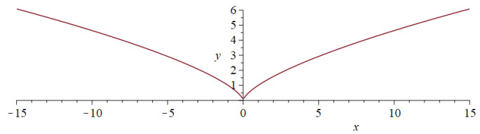
Computer Algebra Systems (CASs) are extremely powerful and widely used digital tools. Focusing on differentiation, CASs include a command that computes the derivative of functions in one variable (and also the partial derivative of functions in several variables). We will focus in this article on real-valued functions of one real variable. Since CASs usually compute the derivative of real-valued functions as a whole, the value of the computed derivative at points where the left derivative and the right derivative are different (that we will call conflicting points) should be something like "undefined", although this isn't always the case: the output could strongly differ depending on the chosen CAS. We have analysed and compared in this article how some well-known CASs behave when addressing differentiation at the conflicting points of five different functions chosen by the authors. Finally, the ability for calculating one-sided limits of CASs allows to directly compute the result in these cumbersome cases using the formal definition of one-sided derivative, which we have also analysed and compared for the selected CASs. Regarding teaching, this is an important issue, as it is a topic of Secondary Education and nowadays the use of CASs as an auxiliary digital tool for teaching mathematics is very common.
- computer algebra systems,
- one-sided differentiability,
- real-valued functions of one real variable,
- limits,
- software comparison
Citation: Enrique Ferres-López, Eugenio Roanes-Lozano, Angélica Martínez-Zarzuelo, Fernando Sánchez. One-sided differentiability: a challenge for computer algebra systems[J]. Electronic Research Archive, 2023, 31(3): 1737-1768. doi: 10.3934/era.2023090

Related Papers:

Abstract

Computer Algebra Systems (CASs) are extremely powerful and widely used digital tools. Focusing on differentiation, CASs include a command that computes the derivative of functions in one variable (and also the partial derivative of functions in several variables). We will focus in this article on real-valued functions of one real variable. Since CASs usually compute the derivative of real-valued functions as a whole, the value of the computed derivative at points where the left derivative and the right derivative are different (that we will call conflicting points) should be something like "undefined", although this isn't always the case: the output could strongly differ depending on the chosen CAS. We have analysed and compared in this article how some well-known CASs behave when addressing differentiation at the conflicting points of five different functions chosen by the authors. Finally, the ability for calculating one-sided limits of CASs allows to directly compute the result in these cumbersome cases using the formal definition of one-sided derivative, which we have also analysed and compared for the selected CASs. Regarding teaching, this is an important issue, as it is a topic of Secondary Education and nowadays the use of CASs as an auxiliary digital tool for teaching mathematics is very common.

References

[1]	E. Ferres-López, E. Roanes-Lozano, Una breve nota didáctica sobre la evaluación de funciones fuera de su dominio usando software matemático, Boletín de la Sociedad Puig Adam, 113 (2022), 71–80.
[2]	E. Ferres-López, E. Roanes-Lozano, A. Martínez-Zarzuelo, Limit calculation outside the domain of definition of real functions using computer algebra systems: an educational panoramic view, in Proceedings of the 27th Asian Technology Conference in Mathematics, (2022), 372–382. Available from: https://atcm.mathandtech.org/EP2022/regular/21979.pdf.
[3]	PlanetMath, One-sided derivatives, 2013. Available from: https://planetmath.org/onesidedderivatives.
[4]	B. Rubio, Funciones de Variable Real, Madrid, España, 2006.
[5]	K. R. Stromberg, An Introduction to Classical Real Analysis, AMS Clesea Publishing, Providence, RI, USA, 1981.
[6]	F. Sánchez, Apuntes de Cálculo I, (n.a.). Available from: http://matematicas.unex.es/fsanchez/calculoI/.
[7]	R. J. Iraundegui, Descartes 2D—Existencia de la Derivada, (n.a.). Available from: http://recursostic.educacion.es/descartes/web/materiales_didacticos/Derivadas_y_derivadas_later-ales/derivadas3.htm.
[8]	J. A. Méndez Contreras, Utilización de Maple como apoyo a la matemática en el Bachillerato, Federación Española de Sociedades de Profesores de Matemáticas (FESPM), Colección Cuadernos para el aula. Badajoz, Spain, 2002.
[9]	E. Ferres-López, E. R. Lozano, A. M. Zarzuelo, Approach to the one-sided differentiability concept with a computer algebra system from the point of view of mathematics education, in CADGME Conference—Digital Tools in Mathematics Education, Abstracts, (2022), 30–31. Available from: https://drive.google.com/file/d/1qF4ceMg6gNklOPa1JVkgKND1dOqNmyka/view.
[10]	Wikipedia, List of computer algebra systems, 2022. Available from: https://en.wikipedia.org/wiki/List_of_computer_algebra_systems.
[11]	L. Bernardin, P. Chin, P. DeMarco, K. O. Geddes, D. E. G. Hare, K. M. Heal, et al., Maple Programming Guide, Maplesoft, Waterloo Maple Inc. Waterloo, Canada, 2020. Available from: https://www.maplesoft.com/documentation_center/Maple2021/ProgrammingGuide.pdf.
[12]	R. M. Corless, Essential Maple—An Introduction for Scientific Programmers, Springer, New York, NY, USA, 1995. https://doi.org/10.1007/978-1-4757-3985-5
[13]	Maplesoft, Maple User Manual, Maplesoft, Waterloo Maple Inc. Waterloo, ON, Canada, 2022. Available from: https://www.maplesoft.com/documentation_center/maple2022/UserManual.pdf.
[14]	E. Roanes-Macías, E. Roanes-Lozano, Cálculos Matemáticos por Ordenador con Maple V.5., Editorial Rubiños-1890, Madrid, España, 1999.
[15]	J. R. Sendra, S. Pérez-Díaz, J. Sendra, C. Villarino, Introducción a la Computación Simbólica y Facilidades Maple, Ra-Ma, Madrid, España, 2012.
[16]	Maplesoft, Maple Product History, (n.a.). Available from: https://www.maplesoft.com/products/maple/history/.
[17]	Maplesoft, Geometry Homework Help: Use Maple 10 to help with your geometry homework and assignments, (n.a.). Available from: https://www.maplesoft.com/maple10/maple10_students-geometry.aspx.
[18]	B. Kutzler, V. Kokol-Voljc, Introduction to Derive 6, Kutzler & Kokol-Voljc OEG, Austria, 2003.
[19]	E. Roanes-Lozano, J. L. Galán-García, C. Solano-Macías, Some reflections about the success and impact of the computer algebra system Derive with a 10-year time perspective, Math. Comput. Sci., 13 (2019), 417–431. https://doi.org/10.1007/s11786-019-00404-9 doi: 10.1007/s11786-019-00404-9
[20]	Maxima—A Computer Algebra System, 2022. Available from: https://maxima.sourceforge.io/.
[21]	J. E. Villate, XMaxima Manual, 2006. Available from: https://maxima.sourceforge.io/docs/xmaxima/xmaxima.pdf.
[22]	Wolfram Alpha, (n.a.). Available from: https://www.wolframalpha.com/.
[23]	J. B. Cassel, Wolfram\|Alpha: a computational knowledge "Search" engine, in Google It (ed. N. Lee), (2016), 267–299. https://doi.org/10.1007/978-1-4939-6415-4_11
[24]	Wolfram Mathematica—Comparative Analysis, Computer Algebra Systems. Available from: https://www.wolfram.com/mathematica/analysis/content/ComputerAlgebraSystems.html.
[25]	J. A. Moraño-Fernández, L. M. Sánchez-Ruiz, Cálculo y Álgebra con Mathematica 10, Universitat Politècnica de València, Valencia, España, 2015.
[26]	Wolfram Language & System—Documentation Center. Available from: https://reference.wolfram.com/language/?source=nav.
[27]	Wolfram Mathematica—Fast introduction for math students, (n.a.). Available from: https://www.wolfram.com/language/fast-introduction-for-math-students/es/?source=footer.
[28]	Sage, Documentation, (n.a.). Available from: SageMath Documentation. https://doc.sagemath.org/.
[29]	The Sage Development Team, Sage Reference Manual, 2022. Available from: https://doc.sagemath.org/html/en/reference/index.html.
[30]	SymPy Documentation Release 1.10.1., 2022. Available from: https://github.com/sympy/sympy/releases.
[31]	GeoGebra Classic Manual, (n.a.). Available from: https://wiki.geogebra.org/en/Libro.
[32]	H. Kronk, Despite clearing 100 million users, GeoGebra remains true to its founder's vision, 2018. Available from: https://news.elearninginside.com/despite-clearing-100-million-users-geogebra-remains-true-to-its-founders-vision/.
[33]	REDUCE, What is REDUCE, (n.a.). Available from: https://reduce-algebra.sourceforge.io/.
[34]	G. Rayna, REDUCE—Software for Algebraic Computation, Springer-Verlag, New York, 1987. https://doi.org/10.1007/978-1-4612-4806-4
[35]	M. McCallum, F. Wright, Algebraic Computing with REDUCE, Oxford University Pres, Oxford, UK, 1991.
[36]	Axiom, The Scientific Computation System, 2015. Available from: bhttp://www.axiom-developer.org/.
[37]	XCAS Documentation, (n.a.). Available from: https://xcas.univ-grenoble-alpes.fr/documentation/EN.html.
[38]	D. R. Stoutemyer, Crimes and misdemeanors in the computer algebra trade, Not. Am. Math. Soc., 38 (1991), 778–785. Available from: https://www.ams.org/journals/notices/199109/199109FullIssue.pdf.
[39]	J. H. Davenport, The challenges of multivalued "Functions", in Intelligent Computer Mathematics, (2010), 1–12. https://doi.org/10.1007/978-3-642-14128-7_1
[40]	R. M. Corless, D. J. Jeffrey, S. M. Watt, J. H. Davenport, "According to Abramowitz and Stegun" or arccoth needn't be uncouth, ACM SIGSAM Bull., 34 (2000), 58–65. https://doi.org/10.1145/362001.362023 doi: 10.1145/362001.362023
[41]	M. England, R. Bradford, J. H. Davenport, D. Wilson, Understanding branch cuts of expressions, in International Conference on Intelligent Computer Mathematics, (2013), 136–151. https://doi.org/10.1007/978-3-642-39320-4_9
[42]	M. England, E. Cheb-Terrab, R. Bradford, J. H. Davenport, D. Wilson, Branch cuts in maple 17, ACM Commun. Comput. Algebra, 48 (2014), 24–27. https://doi.org/10.1145/2644288.2644293 doi: 10.1145/2644288.2644293
[43]	H. Aslaksen, Can Your Computer Do Complex Analysis? Comput. Algebra Syst. Pract. Guide, (1999), 246–258.
[44]	M. J. Wester, A Critique of the Mathematical Abilities of CA Systems, Comput. Algebra Syst. Pract. Guide, 16 (1999), 25–60.
[45]	L. Bernardin, A review of symbolic solvers, ACM SIGSAM Bull., 30 (1996), 9–20. https://doi.org/10.1145/231191.231193 doi: 10.1145/231191.231193
[46]	J. Monaghan, S. Sun, D. Tall, Construction of the limit concept with a computer algebra system, in Proceedings of the 18th Conference of the International Group for the Psychology of Mathematics Education, (1994), 279–286. Available from: https://citeseerx.ist.psu.edu/document?repid=rep1&type=pdf&doi=332da54b21d4ac7877121501f8ce0cae6fe6a343.
[47]	Mathematica Stack Exchange, What does True mean in this case? 2007. Available from: https://mathematica.stackexchange.com/questions/155021/what-does-true-mean-in-this-case.

Reader Comments

Your name:*

Email:*
© 2023 the Author(s), licensee AIMS Press. This is an open access article distributed under the terms of the Creative Commons Attribution License (http://creativecommons.org/licenses/by/4.0)