On the driver's stochastic nature in car-following behavior: Modeling and stabilizing based on the V2I environment

Ying Luo; Yanyan Chen; Kaiming Lu; Jian Zhang; Tao Wang; Zhiyan Yi; Ying Luo; Yanyan Chen; Kaiming Lu; Jian Zhang; Tao Wang; Zhiyan Yi

doi:10.3934/era.2023017

Electronic Research Archive

2023, Volume 31, Issue 1: 342-366. doi: 10.3934/era.2023017

Previous Article Next Article

Research article

On the driver's stochastic nature in car-following behavior: Modeling and stabilizing based on the V2I environment

1.
Beijing Key Laboratory of Traffic Engineering, Beijing University of Technology, Beijing 100124, China
2.
School of Vehicle and Mobility, Tsinghua University, Beijing 100084, China
3.
Department of Civil & Environmental Engineering, University of Utah, Salt Lake City, UT 84112, United States of America

Received: 22 August 2022 Revised: 17 October 2022 Accepted: 20 October 2022 Published: 02 November 2022

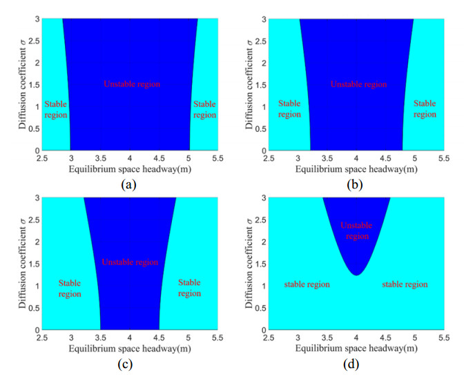
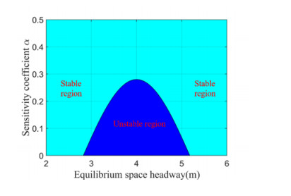
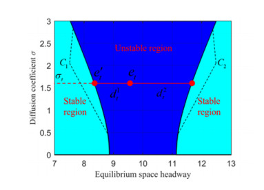
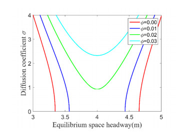
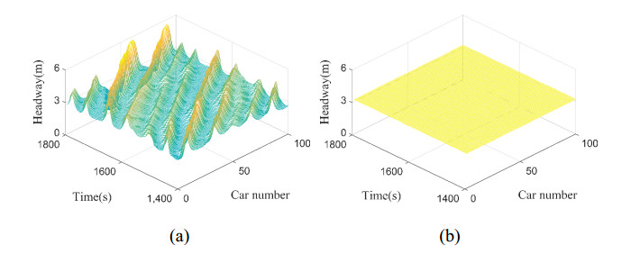
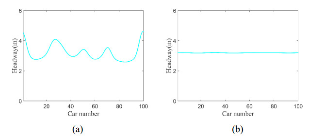
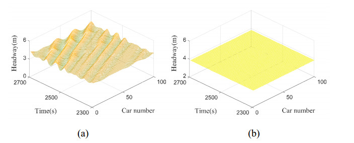
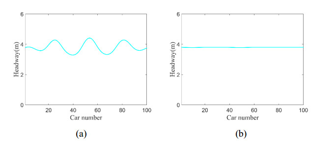
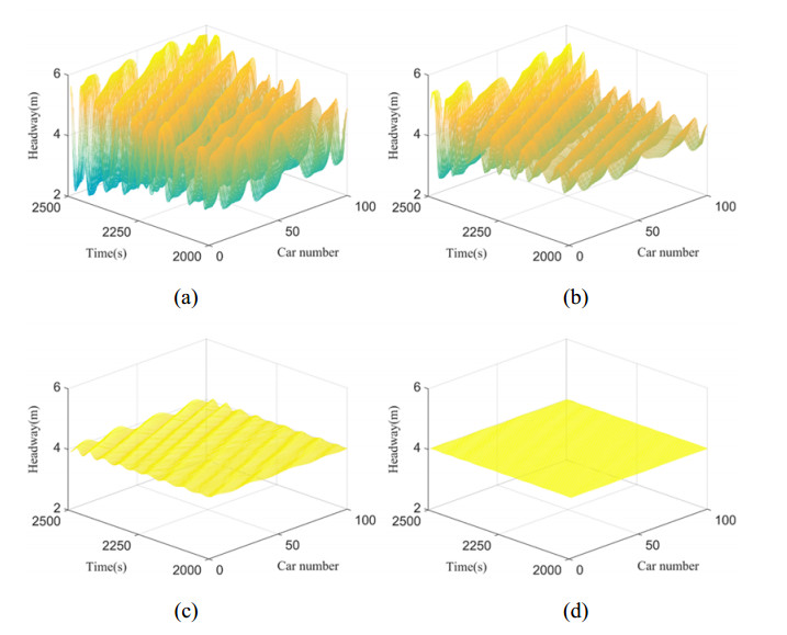
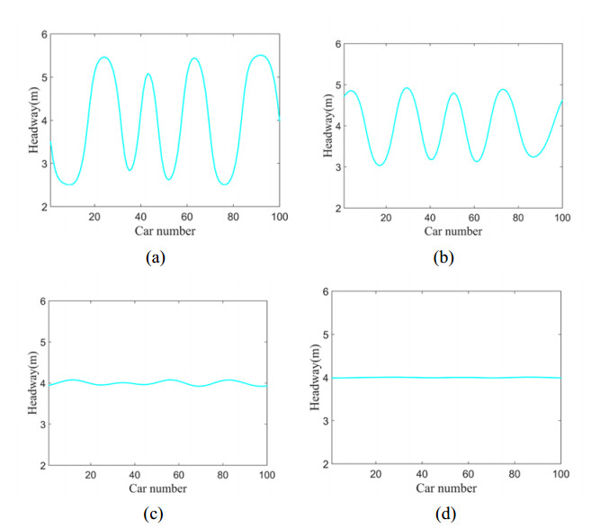
The driver's stochastic nature is one of the important causes of traffic oscillation. To better describe the impact of the driver's stochastic characteristics on car-following behavior, we propose a stochastic full velocity difference model (SFVDM) considering the stochastic variation of the desired velocity. In order to mitigate traffic oscillation caused by driving stochasticity, we further propose a stable speed guidance model (S-SFVDM) by leveraging vehicle-to-infrastructure communication. Stochastic linear stability conditions are derived to demonstrate the prominent influence of the driver's stochasticity on the stability of traffic flow and the improvement of traffic flow stability by the proposed guidance strategy, respectively. We present numerical tests to demonstrate the effectiveness of the proposed models. The results show that the SFVDM can capture the traffic oscillation caused by the driver's stochastic desired velocity and reproduce the same disturbance growth pattern as in the field experiment. The results also indicate that the S-SFVDM can significantly expand the stable area of traffic flow to decrease the negative impact on traffic flow stability caused by the driver's stochastic nature.
- stochastic car-following model,
- stochastic stability analysis,
- V2I environment,
- stable control
Citation: Ying Luo, Yanyan Chen, Kaiming Lu, Jian Zhang, Tao Wang, Zhiyan Yi. On the driver's stochastic nature in car-following behavior: Modeling and stabilizing based on the V2I environment[J]. Electronic Research Archive, 2023, 31(1): 342-366. doi: 10.3934/era.2023017

Related Papers:

Abstract

The driver's stochastic nature is one of the important causes of traffic oscillation. To better describe the impact of the driver's stochastic characteristics on car-following behavior, we propose a stochastic full velocity difference model (SFVDM) considering the stochastic variation of the desired velocity. In order to mitigate traffic oscillation caused by driving stochasticity, we further propose a stable speed guidance model (S-SFVDM) by leveraging vehicle-to-infrastructure communication. Stochastic linear stability conditions are derived to demonstrate the prominent influence of the driver's stochasticity on the stability of traffic flow and the improvement of traffic flow stability by the proposed guidance strategy, respectively. We present numerical tests to demonstrate the effectiveness of the proposed models. The results show that the SFVDM can capture the traffic oscillation caused by the driver's stochastic desired velocity and reproduce the same disturbance growth pattern as in the field experiment. The results also indicate that the S-SFVDM can significantly expand the stable area of traffic flow to decrease the negative impact on traffic flow stability caused by the driver's stochastic nature.

References

[1]	G. F. Newell, Nonlinear effects in the dynamics of car following, Oper. Res., 9 (1961), 209–229.
[2]	M. Bando, K. Hasebe, A. Nakayama, Y. Shibata, Y. Sugiyama, Dynamical model of traffic congestion and numerical simulation, Phys. Rev. E, 51 (1995), 1035. https://doi.org/10.1103/PhysRevE.51.1035 doi: 10.1103/PhysRevE.51.1035
[3]	D. Helbing, B. Tilch, Generalized force model of traffic dynamics, Phys. Rev. E, 58 (1998), 133. https://doi.org/10.1103/PhysRevE.58.133 doi: 10.1103/PhysRevE.58.133
[4]	R. Jiang, Q. Wu, Z. Zhu, Full velocity difference model for a car-following theory, Phys. Rev. E, 64 (2001), 017101. https://doi.org/10.1103/PhysRevE.64.017101 doi: 10.1103/PhysRevE.64.017101
[5]	S. Yu, Z. Shi, Dynamics of connected cruise control systems considering velocity changes with memory feedback, Measurement, 64 (2015), 34–48. https://doi.org/10.1016/j.measurement.2014.12.036 doi: 10.1016/j.measurement.2014.12.036
[6]	J. Chen, R. Liu, D. Ngoduy, Z. K. Shi, A new multi-anticipative car-following model with consideration of the desired following distance, Nonlinear Dyn., 85 (2016), 2705–2717. https://doi.org/10.1007/s11071-016-2856-4 doi: 10.1007/s11071-016-2856-4
[7]	C. Jiang, R. Cheng, H. Ge, An improved lattice hydrodynamic model considering the "backward looking" effect and the traffic interruption probability, Nonlinear Dyn., 91 (2018), 777–784. https://doi.org/10.1007/s11071-017-3908-0 doi: 10.1007/s11071-017-3908-0
[8]	T. Tang, H. Huang, S. Zhao, G. Xu, An extended OV model with consideration of driver's memory, Int. J. Mod. Phys. B., 23 (2009), 743–752. https://doi.org/10.1142/S0217979209051966 doi: 10.1142/S0217979209051966
[9]	D. Liu, Z. Shi, W. H. Ai, Enhanced stability of car-following model upon incorporation of short-term driving memory, Commun. Nonlinear Sci. Numer. Simul., 47 (2017), 139–150. https://doi.org/10.1016/j.cnsns.2016.11.007 doi: 10.1016/j.cnsns.2016.11.007
[10]	S. Yu, J. Tang, Q. Xin, Relative velocity difference model for the car-following theory, Nonlinear Dyn., 91 (2018), 1415–1428. https://doi.org/10.1007/s11071-017-3953-8 doi: 10.1007/s11071-017-3953-8
[11]	S. Yu, M. Huang, J. Ren, Z. Shi, An improved car-following model considering velocity fluctuation of the immediately ahead car, Physica A, 449 (2016), 1–17. https://doi.org/10.1016/j.physa.2015.12.040 doi: 10.1016/j.physa.2015.12.040
[12]	S. Yu, Z. Shi, An improved car-following model considering headway changes with memory, Physica A, 421 (2015), 1–14. https://doi.org/10.1016/j.physa.2014.11.008 doi: 10.1016/j.physa.2014.11.008
[13]	C. Chen, R. Cheng, H. Ge, An extended car-following model considering driver's sensory memory and the backward looking effect, Physica A, 525 (2019), 278–289. https://doi.org/10.1016/j.physa.2019.03.099 doi: 10.1016/j.physa.2019.03.099
[14]	Y. Wang, H. Song, R. Cheng, TDGL and mKdV equations for an extended car-following model with the consideration of driver's memory, Physica A, 515 (2019), 440–449. https://doi.org/10.1016/j.physa.2018.09.171 doi: 10.1016/j.physa.2018.09.171
[15]	R. Sipahi, F. M. Atay, S. I. Niculescu, Stability of traffic flow behavior with distributed delays modeling the memory effects of the drivers, SIAM J. Appl. Math., 68 (2008), 738–759. https://doi.org/10.1137/060673813 doi: 10.1137/060673813
[16]	Y. Chang, Z. He, R. Cheng, An extended lattice hydrodynamic model considering the driver's sensory memory and delayed-feedback control, Physica A, 514 (2008), 522–532. https://doi.org/10.1016/j.physa.2018.09.097 doi: 10.1016/j.physa.2018.09.097
[17]	Y. Sun, H. Ge, R. Cheng, An extended car-following model considering driver's memory and average speed of preceding vehicles with control strategy, Physica A, 521 (2019), 752–761. https://doi.org/10.1016/j.physa.2019.01.092 doi: 10.1016/j.physa.2019.01.092
[18]	Z. Xin, J. Xu, Analysis of a car-following model with driver memory effect, Int. J. Bifurcation Chaos, 25 (2015), 1550057. https://doi.org/10.1142/S0218127415500571 doi: 10.1142/S0218127415500571
[19]	C. Zhai, W. Wu, A new continuum model with driver's continuous sensory memory and preceding vehicle's taillight, Commun. Theor. Phys., 72 (2020), 105004.
[20]	M. Zhou, X. Qu, X. Li, A recurrent neural network based microscopic car following model to predict traffic oscillation, Transp. Res. Part C Emerging Technol., 84 (2017), 245–264. https://doi.org/10.1016/j.trc.2017.08.027 doi: 10.1016/j.trc.2017.08.027
[21]	X. Pei, Y. Pan, H. Wang, S. Wong, K. Choi, Empirical evidence and stability analysis of the linear car-following model with gamma-distributed memory effect, Physica A, 449 (2016), 311–323. https://doi.org/10.1016/j.physa.2015.12.104 doi: 10.1016/j.physa.2015.12.104
[22]	R. Sipahi, F. M. Atay, S. I. Niculescu, Stability of traffic flow behavior with distributed delays modeling the memory effects of the drivers, SIAM J. Appl. Math., 68 (2008), 738–759. https://doi.org/10.1137/060673813 doi: 10.1137/060673813
[23]	M. A. Hossain, J. Tanimoto, The "backward-looking" effect in the continuum model considering a new backward equilibrium velocity function, Nonlinear Dyn., 106 (2021), 2061–2072. https://doi.org/10.1007/s11071-021-06894-2 doi: 10.1007/s11071-021-06894-2
[24]	D. Jia, D. Ngoduy, Enhanced cooperative car-following traffic model with the combination of V2V and V2I communication, Transp. Res. Part B Methodol., 90 (2016), 172–191. https://doi.org/10.1016/j.trb.2016.03.008 doi: 10.1016/j.trb.2016.03.008
[25]	J. Xiao, M. Ma, S. Liang, G. Ma, The non-lane-discipline-based car-following model considering forward and backward vehicle information under connected environment, Nonlinear Dyn., 107 (2022), 2787–2801. https://doi.org/10.1007/s11071-021-06999-8 doi: 10.1007/s11071-021-06999-8
[26]	D. Ngoduy, Analytical studies on the instabilities of heterogeneous intelligent traffic flow, Commun. Nonlinear Sci. Numer. Simul., 18 (2013), 2699–2706. https://doi.org/10.1016/j.cnsns.2013.02.018 doi: 10.1016/j.cnsns.2013.02.018
[27]	J. Larsson, M. F. Keskin, B. Peng, B. Kulcsár, H. Wymeersch, Pro-social control of connected automated vehicles in mixed-autonomy multi-lane highway traffic, Commun. Transp. Res., 1 (2021), 100019. https://doi.org/10.1016/j.commtr.2021.100019 doi: 10.1016/j.commtr.2021.100019
[28]	Y. Li, W. Chen, S. Peeta, Y. Wang, Platoon control of connected multi-vehicle systems under V2X communications: design and experiments, IEEE Trans. Intell. Transp. Syst., 21 (2019), 1891–1902.
[29]	D. Ngoduy, Effect of the car-following combinations on the instability of heterogeneous traffic flow, Transportmetrica B Transport Dyn., 3 (2015), 44–58. https://doi.org/10.1080/21680566.2014.960503 doi: 10.1080/21680566.2014.960503
[30]	B. Wang, T. M. Adams, W. Jin, Q. Meng, The process of information propagation in a traffic stream with a general vehicle headway: A revisit, Transp. Res. Part C Emerging Technol., 18 (2010), 367–375. https://doi.org/10.1016/j.trc.2009.05.011 doi: 10.1016/j.trc.2009.05.011
[31]	X. Wang, Modeling the process of information relay through inter-vehicle communication, Transp. Res. Part B Methodol., 41 (2007), 684–700. https://doi.org/10.1016/j.trb.2006.11.002 doi: 10.1016/j.trb.2006.11.002
[32]	W. Jin, W. W. Recker, Instantaneous information propagation in a traffic stream through inter-vehicle communication, Transp. Res. Part B Methodol., 40 (2006), 230–250. https://doi.org/10.1016/j.trb.2005.04.001 doi: 10.1016/j.trb.2005.04.001
[33]	A. Kesting, M. Treiber, D. Helbing, Enhanced intelligent driver model to access the impact of driving strategies on traffic capacity, Philos. Trans. R. Soc. A Math. Phys. Eng. Sci., 368 (2010), 4585–4605. https://doi.org/10.1098/rsta.2010.0084 doi: 10.1098/rsta.2010.0084
[34]	Y. Li, L. Zhang, S. Peeta, X. He, T. Zheng, Y. Li, A car-following model considering the effect of electronic throttle opening angle under connected environment, Nonlinear Dyn., 85 (2016), 2115–2125. https://doi.org/10.1007/s11071-016-2817-y doi: 10.1007/s11071-016-2817-y
[35]	J. Wu, X. Qu, Intersection control with connected and automated vehicles: a review, J. Intell. and Connected Veh., 5 (2022), 260–269. https://doi.org/10.1108/JICV-06-2022-0023 doi: 10.1108/JICV-06-2022-0023
[36]	T. Olovsson, T. Svensson, J. Wu, Future connected vehicles: Communications demands, privacy and cyber-security, Commun. Transp. Res., 2 (2022), 100056. https://doi.org/10.1016/j.commtr.2022.100056 doi: 10.1016/j.commtr.2022.100056
[37]	K. L. Lim, J. Whitehead, D. Jia, Z. Zheng, State of data platforms for connected vehicles and infrastructures, Commun. Transp. Res., 1 (2021), 10001. https://doi.org/10.1016/j.commtr.2021.100013 doi: 10.1016/j.commtr.2021.100013
[38]	D. Ngoduy, S. Lee, M. Treiber, H. Vu, Langevin method for a continuous stochastic car-following model and its stability conditions, Transp. Res. Part C Emerging Technol., 105 (2019), 599–610. https://doi.org/10.1016/j.trc.2019.06.005 doi: 10.1016/j.trc.2019.06.005
[39]	R. Jiang, M. Hu, H. Zhang, Z. Gao, B. Jia, Q. Wu, et al., Traffic experiment reveals the nature of car-following, PloS One., 9 (2014), 94351. https://doi.org/10.1371/journal.pone.0094351 doi: 10.1371/journal.pone.0094351
[40]	R. Jiang, M. Hu, H. Zhang, Z. Gao, B. Jia, Q. Wu, On some experimental features of car-following behavior and how to model them, Transp. Res. Part B Methodol., 80 (2015), 338–354. https://doi.org/10.1016/j.trb.2015.08.003 doi: 10.1016/j.trb.2015.08.003
[41]	R. Jiang, C. Jin, H. Zhang, Y. Huang, J. Tian, W. Wang, et al., Experimental and empirical investigations of traffic flow instability, Transp. Res. Part C Emerging Technol., 94 (2018), 83–98. https://doi.org/10.1016/j.trc.2017.08.024 doi: 10.1016/j.trc.2017.08.024
[42]	J. Tian, R. Jiang, B. Jia, Z. Gao, S. Ma, Empirical analysis and simulation of the concave growth pattern of traffic oscillations, Transp. Res. Part B Methodol., 93 (2016), 338–354. https://doi.org/10.1016/j.trb.2016.08.001 doi: 10.1016/j.trb.2016.08.001
[43]	J. Tian, H. Zhang, M. Treiber, R. Jiang, Z. Gao, B. Jia, On the role of speed adaptation and spacing indifference in traffic instability: Evidence from car-following experiments and its stochastic model, Transp. Res. Part B Methodol., 129 (2019), 334–350. https://doi.org/10.1016/j.trb.2019.09.014 doi: 10.1016/j.trb.2019.09.014
[44]	F. Zheng, S. E. Jabari, H. Liu, D. Liu, Traffic state estimation using stochastic Lagrangian dynamics, Transp. Res. Part B Methodol., 115 (2018), 143–165. https://doi.org/10.1016/j.trb.2018.07.004 doi: 10.1016/j.trb.2018.07.004
[45]	J. A. Laval, C. S. Toth, Y. Zhou, A parsimonious model for the formation of oscillations in car-following models, Transp. Res. Part B Methodol., 70 (2014), 228–238. https://doi.org/10.1016/j.trb.2014.09.004 doi: 10.1016/j.trb.2014.09.004
[46]	K. Yuan, J. Laval, V. L. Knoop, R. Jiang, S. P. Hoogendoorn, A geometric Brownian motion car-following model: towards a better understanding of capacity drop, Transportmetrica B Transport Dyn., 21 (2018), 915–927. https://doi.org/10.1080/21680566.2018.1518169 doi: 10.1080/21680566.2018.1518169
[47]	J. Tian, C. Zhu, D. Chen, R. Jiang, G. Wang, Z. Gao, Car following behavioral stochasticity analysis and modeling: Perspective from wave travel time, Transp. Res. Part B Methodol., 143 (2021), 160–176. https://doi.org/10.1016/j.trb.2020.11.008 doi: 10.1016/j.trb.2020.11.008
[48]	D. Ngoduy, Noise-induced instability of a class of stochastic higher order continuum traffic models, Transp. Res. Part B Methodol., 150 (2021), 260–278. https://doi.org/10.1016/j.trb.2021.06.013 doi: 10.1016/j.trb.2021.06.013
[49]	P. Lin, X. Liu, M. Pei, P. Wu, Revealing the spatial variation in vehicle travel time with weather and driver travel frequency impacts: Findings from the Guangdong-Hong Kong-Macao Greater Bay Area, China, Electron. Res. Arch., 30 (2022), 3711–3734. https://doi.org/10.3934/era.2022190 doi: 10.3934/era.2022190
[50]	P. Wagner, A time-discrete harmonic oscillator model of human car-following, Eur. Phys. J. B, 84 (2011), 713–718. https://doi.org/10.1140/epjb/e2011-20722-8 doi: 10.1140/epjb/e2011-20722-8
[51]	P. Wagner, Analyzing fluctuations in car-following, Transp. Res. Part B Methodol., 46 (2012), 1384–1392. https://doi.org/10.1016/j.trb.2012.06.007 doi: 10.1016/j.trb.2012.06.007
[52]	M. Makridis, L. Leclercq, B. Ciuffo, G. Fontaras, K. Mattas, Formalizing the heterogeneity of the vehicle-driver system to reproduce traffic oscillations, Transp. Res. Part C Emerging Technol., 120 (2020), 102803. https://doi.org/10.1016/j.trc.2020.102803 doi: 10.1016/j.trc.2020.102803
[53]	J. Wen, C. Wu, R. Zhang, X. Xiao, N. Nv Y. Shi, Rear-end collision warning of connected automated vehicles based on a novel stochastic local multivehicle optimal velocity model, Accid. Anal. Prev., 148 (2020), 105800. https://doi.org/10.1016/j.aap.2020.105800 doi: 10.1016/j.aap.2020.105800
[54]	X. Mao, Stochastic Differential Equations and Applications, Horwood, Chichester, 2008.
[55]	R. Ortega, Variations on Lyapunov's stability criterion and periodic prey-predator systems, Electron. Res. Arch., 29 (2021), 3995. https://doi.org/10.3934/era.2021069 doi: 10.3934/era.2021069

Reader Comments

Your name:*

Email:*
© 2023 the Author(s), licensee AIMS Press. This is an open access article distributed under the terms of the Creative Commons Attribution License (http://creativecommons.org/licenses/by/4.0)