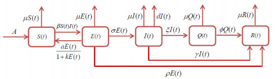
Infectious diseases have a great impact on the economy and society. Dynamic models of infectious diseases are an effective tool for revealing the laws of disease transmission. Quarantine and nonlinear innate immunity are the crucial factors in the control of infectious diseases. Currently, there no mathematical models that comprehensively study the effect of both innate immunity and quarantine. In this paper, we propose and analyze an SEIQR epidemic model with nonlinear innate immunity. The boundedness and positivity of the solutions are discussed. Employing the next-generation matrix, we compute the expression of the basic reproduction number. Under certain conditions, the phenomenon of backward bifurcation may occur. That is to say, the stable disease-free equilibrium point and the stable endemic equilibrium point coexist when the basic reproduction ratio is less than one. And the basic reproduction number is no longer the threshold value to determine whether the disease breaks out. We investigate the globally asymptotical stability of the disease-free equilibrium point for the system by constructing Lyapunov function. Also, we research the global stability of the endemic equilibrium by using geometric approach. Numerical simulations are carried out to reveal the theoretical results and find some complex dynamics (for example, the existence of Hopf bifurcation) of the system. Both theoretical and numerical results indicate that the nonlinear innate immunity may cause backward bifurcation and Hopf bifurcation, which makes more difficult to eliminate the disease.
Citation: Xueyong Zhou, Xiangyun Shi. Stability analysis and backward bifurcation on an SEIQR epidemic model with nonlinear innate immunity[J]. Electronic Research Archive, 2022, 30(9): 3481-3508. doi: 10.3934/era.2022178
Infectious diseases have a great impact on the economy and society. Dynamic models of infectious diseases are an effective tool for revealing the laws of disease transmission. Quarantine and nonlinear innate immunity are the crucial factors in the control of infectious diseases. Currently, there no mathematical models that comprehensively study the effect of both innate immunity and quarantine. In this paper, we propose and analyze an SEIQR epidemic model with nonlinear innate immunity. The boundedness and positivity of the solutions are discussed. Employing the next-generation matrix, we compute the expression of the basic reproduction number. Under certain conditions, the phenomenon of backward bifurcation may occur. That is to say, the stable disease-free equilibrium point and the stable endemic equilibrium point coexist when the basic reproduction ratio is less than one. And the basic reproduction number is no longer the threshold value to determine whether the disease breaks out. We investigate the globally asymptotical stability of the disease-free equilibrium point for the system by constructing Lyapunov function. Also, we research the global stability of the endemic equilibrium by using geometric approach. Numerical simulations are carried out to reveal the theoretical results and find some complex dynamics (for example, the existence of Hopf bifurcation) of the system. Both theoretical and numerical results indicate that the nonlinear innate immunity may cause backward bifurcation and Hopf bifurcation, which makes more difficult to eliminate the disease.

| [1] |
X. Y. Zhou, X. Y. Shi, M. Wei, Dynamical behavior and optimal control of a stochastic mathematical model for cholera, Chaos, Solitons Fractals, 156 (2022), 111854. https://doi.org/10.1016/j.chaos.2022.111854 doi: 10.1016/j.chaos.2022.111854

|
| [2] |
X. Y. Shi, X. W. Gao, X. Y. Zhou, Y. F. Li, Analysis of an SQEIAR epidemic model with media coverage and asymptomatic infection, AIMS Math., 6 (2021), 12298–12320. https://doi.org/10.3934/math.2021712 doi: 10.3934/math.2021712
|
| [3] |
M. Zhao, Y. Zhang, W. T. Li, Y. H. Du, The dynamics of a degenerate epidemic model with nonlocal diffusion and free boundaries, J. Differ. Equations, 269 (2020), 3347–3386. https://doi.org/10.1016/j.jde.2020.02.029 doi: 10.1016/j.jde.2020.02.029
|
| [4] | D. Bernoulli, Essai d'une nouvelle analyse de la mortalité causée par la petite vérole, et des avantages de l'inoculation pour la prévenir, Hist. Acad. R. Sci. M¨¦m. Math. Phys., 1 (1760), 1–45. |
| [5] |
Q. Lin, S. Zhao, D. Gao, Y. Lou, S. Yang, S. S. Musa, et al., A conceptual model for the coronavirus disease 2019 (COVID-19) outbreak in Wuhan, China with individual reaction and governmental action, Int. J. Infect. Dis., 93 (2020), 211–216. https://doi.org/10.1016/j.ijid.2020.02.058 doi: 10.1016/j.ijid.2020.02.058
|
| [6] |
U. Avila-Ponce de Le$\acute{o}$n, $\acute{A}$. G. C. P$\acute{e}$rez, E. Avila-Vales, An SEIARD epidemic model for COVID-19 in Mexico: mathematical analysis and state-level forecast, Chaos, Solitons Fractals, 140 (2020), 110165. https://doi.org/10.1016/j.chaos.2020.110165 doi: 10.1016/j.chaos.2020.110165
|
| [7] |
J. K. K. Asamoah, F. Nyabadza, Z. Jin, E. Bonyah, M. A. Khan, M. Y. Li, et al., Backward bifurcation and sensitivity analysis for bacterial meningitis transmission dynamics with a nonlinear recovery rate, Chaos, Solitons Fractals, 140 (2020), 110237. https://doi.org/10.1016/j.chaos.2020.110237 doi: 10.1016/j.chaos.2020.110237
|
| [8] |
N. Chitnis, J. M. Cushing, J. M. Hyman, Bifurcation analysis of a mathematical model for malaria transmission, SIAM J. Appl. Math., 67 (2006), 24–45. https://doi.org/10.1137/050638941 doi: 10.1137/050638941
|
| [9] |
I. Al-Darabsah, Y. Yuan, A time-delayed epidemic model for Ebola disease transmission, Appl. Math. Comput., 290 (2016), 307–325. https://doi.org/10.1016/j.amc.2016.05.043 doi: 10.1016/j.amc.2016.05.043
|
| [10] |
S. He, Y. Peng, K. Sun, SEIR modeling of the COVID-19 and its dynamics, Nonlinear Dym., 101 (2020), 1667–1680. https://doi.org/10.1007/s11071-020-05743-y doi: 10.1007/s11071-020-05743-y
|
| [11] |
J. K. K. Asamoah, Z. Jin, G. Q. Sun, B. Seidu, E. Yankson, A. Abidemi, et al., Sensitivity assessment and optimal economic evaluation of a new COVID-19 compartmental epidemic model with control interventions, Chaos, Solitons Fractals, 146 (2021), 110885. https://doi.org/10.1016/j.chaos.2021.110885 doi: 10.1016/j.chaos.2021.110885
|
| [12] |
X. Zhao, X. He, T. Feng, Z. Qiu, A stochastic switched SIRS epidemic model with nonlinear incidence and vaccination: stationary distribution and extinction, Int. J. Biomath., 13 (2020), 2050020. https://doi.org/10.1142/S1793524520500205 doi: 10.1142/S1793524520500205
|
| [13] |
A. Omame, M. Abbas, C. P. Onyenegecha, Backward bifurcation and optimal control in a co-infection model for SARS-CoV-2 and ZIKV, Results Phys., 37 (2022), 105481. https://doi.org/10.1016/j.rinp.2022.105481 doi: 10.1016/j.rinp.2022.105481
|
| [14] |
Y. Zhao, H. Li, W. Li, Y. Wang, Global stability of a SEIR epidemic model with infectious force in latent period and infected period under discontinuous treatment strategy, Int. J. Biomath., 14 (2021), 2150034. https://doi.org/10.1016/j.chaos.2004.11.062 doi: 10.1016/j.chaos.2004.11.062
|
| [15] |
H. Herbert, Z. E. Ma, S. B. Liao, Effects of quarantine in six endemic models for infectious diseases, Math. Biosci., 180 (2002), 141–160. https://doi.org/10.1016/S0025-5564(02)00111-6 doi: 10.1016/S0025-5564(02)00111-6
|
| [16] |
M. Ali, S. T. H. Shah, M. Imran, A. Khan, The role of asymptomatic class, quarantine and isolation in the transmission of COVID-19, J. Biol. Dyn., 14 (2020), 389–408. https://doi.org/10.1080/17513758.2020.1773000 doi: 10.1080/17513758.2020.1773000
|
| [17] |
T. W. Tulu, B. Tian, Z. Wu, Modeling the effect of quarantine and vaccination on Ebola disease, Adv. Differ. Equations, 2017 (2017), 1–14. https://doi.org/10.1186/s13662-017-1225-z doi: 10.1186/s13662-017-1225-z
|
| [18] | B. Beutler, Innate immunity: an overview, Mol. Immunol., 40 (2004), 845–859. https://doi.org/10.1016/j.molimm.2003.10.005 |
| [19] |
K. M. A. Kabir, J. Tanimoto, Analysis of individual strategies for artificial and natural immunity with imperfectness and durability of protection, J. Theor. Biol., 509 (2021), 110531. https://doi.org/10.1016/j.jtbi.2020.110531 doi: 10.1016/j.jtbi.2020.110531
|
| [20] |
S. Jain, S. Kumar, Dynamical analysis of SEIS model with nonlinear innate immunity and saturated treatment, Eur. Phys. J. Plus, 136 (2021), 952. https://doi.org/10.1140/epjp/s13360-021-01944-5 doi: 10.1140/epjp/s13360-021-01944-5
|
| [21] |
S. Jain, S. Kumar, Dynamic analysis of the role of innate immunity in SEIS epidemic model, Eur. Phys. J. Plus, 136 (2021), 439. https://doi.org/10.1140/epjp/s13360-021-01390-3 doi: 10.1140/epjp/s13360-021-01390-3
|
| [22] |
N. Yi, Q. Zhang, K. Mao, D. Yang, Q. Li, Analysis and control of an SEIR epidemic system with nonlinear transmission rate, Math. Comput. Modell., 50 (2009), 1498–1513. https://doi.org/10.1016/j.mcm.2009.07.014 doi: 10.1016/j.mcm.2009.07.014
|
| [23] |
R. Almeida, A. B. Cruz, N. Martins, M. T. T. Monteiro, An epidemiological MSEIR model described by the Caputo fractional derivative, Int. J. Dyn. Control, 7 (2019), 776–784. https://doi.org/10.1007/s40435-018-0492-1 doi: 10.1007/s40435-018-0492-1
|
| [24] |
P. van den Driessche, J. Watmough, Reproduction numbers and sub-threshold endemic equilibria for compartmental models of disease transmission, Math. Biosci., 180 (2002), 29–48. https://doi.org/10.1016/S0025-5564(02)00108-6 doi: 10.1016/S0025-5564(02)00108-6
|
| [25] |
C. Castillo-Chavez, B. J. Song, Dynamical models of tubercolosis and their applications, Math. Biosci. Eng., 1 (2004), 361–404. https://doi.org/10.3934/mbe.2004.1.361 doi: 10.3934/mbe.2004.1.361
|
| [26] | J. Guckenheimer, P. Holmes, Nonlinear Oscillations, Dynamical Systems and Bifurcations of Vector Fields, Springer, Berlin, 1983. https://doi.org/10.1007/978-1-4612-1140-2 |
| [27] |
J. Arino, C. C. McCluskey, P. van den Driessche, Global results for an epidemic model with vaccination that exhibits backward bifurcations, SIAM J. Appl. Math., 64 (2003), 260–276. https://doi.org/10.1137/S0036139902413829 doi: 10.1137/S0036139902413829
|
| [28] |
M. Y. Li, J. S. Muldowney, On R. A. Smith's autonomous convergence theorem, Rocky Mount. J. Math., 25 (1995), 365–379. https://doi.org/10.1216/rmjm/1181072289 doi: 10.1216/rmjm/1181072289
|
| [29] |
M. Y. Li, J. S. Muldowney, A geometric approach to globle stability problems, SIAM J. Math. Anal., 27 (1996), 1070–1083. https://doi.org/10.1137/S0036141094266449 doi: 10.1137/S0036141094266449
|
| [30] | M. Y. Li, J. S. Muldowney, On Bendixson's criterion, J. Differ. Equation, 106 (1993), 27–39. https://doi.org/10.1006/jdeq.1993.1097 |
| [31] |
J. S. Muldowney, Compound matrices and ordinary differential equations, Rocky Mount. J. Math., 20 (1990), 857–872. https://doi.org/10.1216/rmjm/1181073047 doi: 10.1216/rmjm/1181073047
|
| [32] |
M. Y. Li, H. L. Smith, L. Wang, Global dynamics of an SEIR epidemic model with vertical transmission, SIAM J. Appl. Math., 62 (2001), 58–69. https://doi.org/10.1137/S0036139999359860 doi: 10.1137/S0036139999359860
|
| [33] | M. Y. Li, J. S. Muldowney, Global stability for the SEIR model in epidemiology, Math. Biosci. 125 (1995), 155–164. https://doi.org/10.1016/0025-5564(95)92756-5 |
| [34] |
A. B. Gumel, C. C. McCluskey, J. Watmough, An SVEIR modelfor assessing potential impact of an imperfect anti-SARS vaccine, Math. Biosci. Eng., 3 (2006), 485–512. https://doi.org/10.3934/mbe.2006.3.485 doi: 10.3934/mbe.2006.3.485
|
| [35] |
X. M. Feng, Z. D. Teng, K. Wang, F. Q. Zhang, Backward bifurcation and global stability in an epidemic model with treatment and vaccination, Discrete Contin. Dyn. Syst., 19 (2014), 999–1025. https://doi.org/10.3934/dcdsb.2014.19.999 doi: 10.3934/dcdsb.2014.19.999
|


Figures(6)
Xueyong Zhou, Xiangyun Shi. Stability analysis and backward bifurcation on an SEIQR epidemic model with nonlinear innate immunity[J]. Electronic Research Archive, 2022, 30(9): 3481-3508. doi: 10.3934/era.2022178


 DownLoad: