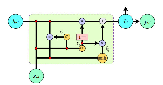
With the rapid development of artificial intelligence technology, the intelligence and autonomy of Unmanned Aerial Vehicles (UAVs) have been significantly improved. Because the real trajectory data is often discontinuous and random, the current aircraft maneuver trajectory prediction methods are far from meeting the practical requirements of the autonomous air tasks. Especially, in order to occupy a better position rapidly where it is easier to attack the enemy, a fast and accurate maneuver trajectory prediction method for the UAVs is proposed in this paper. Firstly, the prediction model of aircraft maneuvering trajectory is built by extracting characteristic information from the historical trajectory. Aiming at the problem of slow optimization speed and easy to fall into local optimization, a global aircraft maneuver trajectory prediction method based on the Hummingbird Optimization Algorithm (HOA) and Gated Recurrent Unit (GRU) is proposed. Then, the implementation process of the maneuver trajectory prediction method based on the above HOA-GRU network for the UAVs is presented. Finally, the aircraft maneuver trajectory prediction method is applied to a simulation training system with the discontinuous and random air task data. The simulation results show that the proposed method can predict the maneuver trajectory of the UAVs with discontinuous data in real time with less error and less time.
Citation: Zhizhou Zhang, Zhenglei Wei, Bowen Nie, Yang Li. Discontinuous maneuver trajectory prediction based on HOA-GRU method for the UAVs[J]. Electronic Research Archive, 2022, 30(8): 3111-3129. doi: 10.3934/era.2022158
With the rapid development of artificial intelligence technology, the intelligence and autonomy of Unmanned Aerial Vehicles (UAVs) have been significantly improved. Because the real trajectory data is often discontinuous and random, the current aircraft maneuver trajectory prediction methods are far from meeting the practical requirements of the autonomous air tasks. Especially, in order to occupy a better position rapidly where it is easier to attack the enemy, a fast and accurate maneuver trajectory prediction method for the UAVs is proposed in this paper. Firstly, the prediction model of aircraft maneuvering trajectory is built by extracting characteristic information from the historical trajectory. Aiming at the problem of slow optimization speed and easy to fall into local optimization, a global aircraft maneuver trajectory prediction method based on the Hummingbird Optimization Algorithm (HOA) and Gated Recurrent Unit (GRU) is proposed. Then, the implementation process of the maneuver trajectory prediction method based on the above HOA-GRU network for the UAVs is presented. Finally, the aircraft maneuver trajectory prediction method is applied to a simulation training system with the discontinuous and random air task data. The simulation results show that the proposed method can predict the maneuver trajectory of the UAVs with discontinuous data in real time with less error and less time.

| [1] |
J. L. Yepes, I. Hwang, M. Rotea, New algorithms for aircraft intent inference and trajectory prediction, J. Guid. Control Dyn., 30 (2012), 370–382. https://doi.org/10.2514/1.26750 doi: 10.2514/1.26750

|
| [2] |
L. Xie, Z. Wei, D. Ding, Z. Zhang, A. Tang, Long and short term maneuver trajectory prediction of UCAV based on deep learning, IEEE Access, 9 (2021), 32321–32340. https://doi.org/10.1109/ACCESS.2021.3060783 doi: 10.1109/ACCESS.2021.3060783
|
| [3] | D. Ding, Z. Wei, S. Tang, Z. Huang, Robust maneuvering decision-making method for air combat using adaptive prediction weight, Syst. Eng. Electron., 42 (2020), 2275–2284. |
| [4] | T. Wang, B. Huang, 4D flight trajectory prediction model based on improved Kalman filter, J. Comput. Appl., 34 (2014), 1812–1815. |
| [5] |
K. Zhang, J. Xiong, Fan. Li, T. Fu, Bayesian trajectory prediction for a hypersonic gliding reentry vehicle based on intent inference, J. Astronaut., 39 (2018), 1258–1265. https://doi.org/10.3873/j.issn.1000-1328.2018.11.008 doi: 10.3873/j.issn.1000-1328.2018.11.008
|
| [6] | L. Wang, Q. Xing, Y. Mao, A track forecasting algorithm of boost-glide unpropulsive skipping vehicle, J. Air Force Eng. Univ. (Nat. Sci. Ed.), 16 (2015), 24–27. |
| [7] |
Q. Wang, Z. Zhang, Z. Wang, Y. Wang, W. Zhou, The trajectory prediction of spacecraft by grey method, Meas. Sci. Technol., 27 (2016), 085011–085020. https://doi.org/10.1088/0957-0233/27/8/085011 doi: 10.1088/0957-0233/27/8/085011
|
| [8] | C. G. Prevost, A. Desbiens, E. Gagnon, Extended kalman filter for state estimation and trajectory prediction of a moving object detected by an unmanned aerial vehicle, in 2007 American Control Conference, (2007), 1805–1810. https://doi.org/10.1109/ACC.2007.4282823 |
| [9] |
G. Li, H. Zhang, G. Tang, Typical trajectory characteristics of hypersonic glide vehicle, J. Astronaut., 36 (2015) 397–403. https://doi.org/10.3873/j.issn.1000-1328.2015.04.005 doi: 10.3873/j.issn.1000-1328.2015.04.005
|
| [10] |
C. Han, J. Xiong, K. Zhang, X. Lan, Decomposition ensemble trajectory prediction algorithm for hypersonic vehicle, Syst. Eng. Electron., 40 (2018), 151–158. https://doi.org/10.3969/j.issn.1001-506X.2018.01.22 doi: 10.3969/j.issn.1001-506X.2018.01.22
|
| [11] |
M. Q. Chen, Aircraft climb trajectory prediction using neural network, Appl. Mech. Mater., 373-375 (2013), 1247–1250. https://doi.org/10.4028/www.scientific.net/AMM.373-375.1247 doi: 10.4028/www.scientific.net/AMM.373-375.1247
|
| [12] |
X. Wang, R. Yang, J. Zuo, X. Xu, L. Yue, Trajectory prediction of target aircraft based on HPSO-TPFENN neural network, J. Northwest. Polytech. Univ., 37 (2019), 612–620. https://doi.org/10.1051/jnwpu/20193730612 doi: 10.1051/jnwpu/20193730612
|
| [13] |
H. Zhang, C. Huang, S. Tang, Y. Xuan, CNN-based real-time prediction method of flight trajectory of unmanned combat aerial vehicle, Acta Armamentarii, 41 (2020), 1894–1903. https://doi.org/10.3969/j.issn.1000-1093.2020.09.022 doi: 10.3969/j.issn.1000-1093.2020.09.022
|
| [14] |
Y. Lecun, Y. Bengio, G. Hinton, Deep learning, Nature, 521 (2015), 436–444. https://doi.org/10.1038/nature14539 doi: 10.1038/nature14539
|
| [15] |
S. L. Churchill, RNN composition of thematically diverse video game melodies, Comput. Games, 8 (2019), 41–58. https://doi.org/10.1007/s40869-018-0063-x doi: 10.1007/s40869-018-0063-x
|
| [16] |
S. Hochreiter, J. Schmidhuber, Long short-term memory, Neural Comput., 9 (1997), 1735–1780. https://doi.org/10.1162/neco.1997.9.8.1735 doi: 10.1162/neco.1997.9.8.1735
|
| [17] | F. Rui, Z. Zuo, L. Li, Using LSTM and GRU neural network methods for traffic flow prediction, in 2016 31st Youth Academic Annual Conference of Chinese Association of Automation (YAC), (2016), 324–328. https://doi.org/10.1109/YAC.2016.7804912 |
| [18] |
Z. Zhang, C. Huang, D. Ding, S. Tang, B. Han, H. Huang, Hummingbirds optimization algorithm-based particle filter for maneuvering target tracking, Nonlinear Dyn., 97 (2019), 1227–1243. https://doi.org/10.1007/s11071-019-05043-0 doi: 10.1007/s11071-019-05043-0
|
| [19] |
Z. Zhang, C. Huang, H. Huang, S. Tang, K. Dong, An optimization method: hummingbirds optimization algorithm, J. Syst. Eng. Electron., 29 (2018), 386–404. https://doi.org/10.21629/JSEE.2018.02.19 doi: 10.21629/JSEE.2018.02.19
|
| [20] |
J. Y. Yoon, A. H. Lee, H. J. Lee, Rendezvous: opportunistic data delivery to mobile users by UAVs through target trajectory prediction, IEEE Trans. Veh. Technol., 69 (2020), 2230–2245. https://doi.org/10.1109/TVT.2019.2962391 doi: 10.1109/TVT.2019.2962391
|
| [21] | B. Hu, H. Yang, L. Wang, S. Chen, A trajectory prediction based intelligent handover control method in UAV cellular networks, China Commun., 16 (2019), 1–14. Available from: https://ieeexplore.ieee.org/document/8633299. |


Figures(7) / Tables(3)
Zhizhou Zhang, Zhenglei Wei, Bowen Nie, Yang Li. Discontinuous maneuver trajectory prediction based on HOA-GRU method for the UAVs[J]. Electronic Research Archive, 2022, 30(8): 3111-3129. doi: 10.3934/era.2022158


 DownLoad: