Designing and tuning MIMO feedforward controllers using iterated LMI restriction

Saeedreza Tofighi; Farshad Merrikh-Bayat; Farhad Bayat; Saeedreza Tofighi; Farshad Merrikh-Bayat; Farhad Bayat

doi:10.3934/era.2022126

Electronic Research Archive

2022, Volume 30, Issue 7: 2465-2486. doi: 10.3934/era.2022126

Previous Article Next Article

Research article

Designing and tuning MIMO feedforward controllers using iterated LMI restriction

Department of Electrical and Computer Engineering, University of Zanjan, University Blvd., Zanjan 45371-38791, Iran

Academic Editor: Predrag Stanimirovic

Received: 29 December 2021 Revised: 18 April 2022 Accepted: 25 April 2022 Published: 29 April 2022

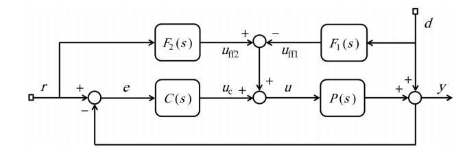
In this paper, a multi-input multi-output (MIMO) feedforward control structure is proposed and designed based on the linear matrix inequality (LMI) approach to improve disturbance rejection and reference tracking of the given feedback system. The proposed architecture consists of two MIMO feedforward controllers, where each controller can be designed independently using the proposed method. The unknown variables of the feedforward controllers are calculated using LMI restrictions such that the H_∞-norm of the transfer function matrix from disturbance (set-point) to output (error) is minimized. By taking advantage of the frequency sampling techniques and using some iterative algorithms, convergence of the solution to a local optimal point is guaranteed. For solving this optimization problem the CVX optimization tool is used and the numerical results are presented. The proposed method can be considered as a new tractable approach for tuning the parameters of MIMO feedforward controllers.
- MIMO feedforward controller,
- disturbance rejection,
- set-point tracking,
- linear matrix inequality (LMI),
- semidefinite program (SDP) optimization
Citation: Saeedreza Tofighi, Farshad Merrikh-Bayat, Farhad Bayat. Designing and tuning MIMO feedforward controllers using iterated LMI restriction[J]. Electronic Research Archive, 2022, 30(7): 2465-2486. doi: 10.3934/era.2022126

Related Papers:

Abstract

In this paper, a multi-input multi-output (MIMO) feedforward control structure is proposed and designed based on the linear matrix inequality (LMI) approach to improve disturbance rejection and reference tracking of the given feedback system. The proposed architecture consists of two MIMO feedforward controllers, where each controller can be designed independently using the proposed method. The unknown variables of the feedforward controllers are calculated using LMI restrictions such that the H_∞-norm of the transfer function matrix from disturbance (set-point) to output (error) is minimized. By taking advantage of the frequency sampling techniques and using some iterative algorithms, convergence of the solution to a local optimal point is guaranteed. For solving this optimization problem the CVX optimization tool is used and the numerical results are presented. The proposed method can be considered as a new tractable approach for tuning the parameters of MIMO feedforward controllers.

References

[1]	L. Consolini, G. Lini, A. Piazzi, A. Visioli, Minimumtime rest-to-rest feedforward action for PID feedback MIMO systems, IFAC Proc. Vol., 45 (2012), 217-222. DOI:10.3182/20120328-3-IT-3014.00037 doi: 10.3182/20120328-3-IT-3014.00037
[2]	F. García-añ as, J. L. Guzmán, F. Rodríguez, M. Berenguel, T. Hä gglund, Experimental evaluation of feedforward tuning rules, IFAC Proc. Vol., 114 (2021), 104877. DOI:10.1016/j.conengprac.2021.104877 doi: 10.1016/j.conengprac.2021.104877
[3]	P. Roy, B. K. Roy, Dual mode adaptive fractional order PI controller with feedforward controller based on variable parameter model for quadruple tank process, ISA Trans., 63 (2016), 365-376. DOI:10.1016/j.isatra.2016.03.010 doi: 10.1016/j.isatra.2016.03.010
[4]	Y. Hamada, Flight test results of disturbance attenuation using preview feedforward compensation, IFAC-PapersOnLine, 50 (2017), 14188-14193. DOI:10.1016/j.ifacol.2017.08.2086 doi: 10.1016/j.ifacol.2017.08.2086
[5]	D. Carnevale, S. Galeani, M. Sassano, Transient optimization in output regulation via feedforward selection and regulator state initialization, IFAC-PapersOnLine, 50 (2017), 2405-8963. DOI:10.1016/j.ifacol.2017.08.677 doi: 10.1016/j.ifacol.2017.08.677
[6]	W. L. Luyben, Comparison of additive and multiplicative feedforward control, J. Process Control, 111 (2022), 1-7. DOI:10.1016/j.jprocont.2022.01.004 doi: 10.1016/j.jprocont.2022.01.004
[7]	Y. Du, W. Cao, J. She, M. Wu, M. Fang, Disturbance rejection via feedforward compensation using an enhanced equivalent-input-disturbance approach, J. Franklin Inst., 357 (2020), 10977-10996. DOI:10.1016/j.jfranklin.2020.05.052 doi: 10.1016/j.jfranklin.2020.05.052
[8]	J. Wu, Y. Han, Z. Xiong, H. Ding, Servo performance improvement through iterative tuning feedforward controller with disturbance compensator, Int. J. Mach. Tools Manuf., 117 (2017), 1-10. DOI:10.1016/j.ijmachtools.2017.02.002 doi: 10.1016/j.ijmachtools.2017.02.002
[9]	Y. Pasco, O. Robin, P. Bélanger, A. Berry, S. Rajan, Multi-input multi-output feedforward control of multi-harmonic gearbox vibrations using parallel adaptive notch filters in the principal component space, J. Sound Vib., 330 (2011), 5230-5244. DOI:10.1016/j.jsv.2011.06.008 doi: 10.1016/j.jsv.2011.06.008
[10]	S. Liu, G. Shi, D. Li, Active disturbance rejection control based on feedforward inverse system for turbofan engines, IFAC-PapersOnLine, 54 (2021), 376-381. DOI:10.1016/j.ifacol.2021.10.191 doi: 10.1016/j.ifacol.2021.10.191
[11]	D. Vrecko, M. Nerat, D. Vrancic, G. Dolanc, B. Dolenc, B. Pregelj, et al., Feedforward-feedback control of a solid oxide fuel cell power system, Int. J. Hydrog. Energy, 43 (2018), 6352-6363. DOI:10.1016/j.ijhydene.2018.01.203 doi: 10.1016/j.ijhydene.2018.01.203
[12]	L. Liu, S. Tian, D. Xue, T. Zhang, Y. Q. Chen, Industrial feedforward control technology: a review, J. Intell. Manuf., 30 (2019), 2819-2833. DOI:10.1007/s10845-018-1399-6 doi: 10.1007/s10845-018-1399-6
[13]	M. N. A. Parlakci, E. M. Jafarov, A robust delay-dependent guaranteed cost PID multivariable output feedback controller design for time-varying delayed systems: An LMI optimization approach, Eur. J. Control, 61 (2021), 68-79. DOI:10.1016/j.ejcon.2021.06.003 doi: 10.1016/j.ejcon.2021.06.003
[14]	Z. Y. Feng, H. Guo, J. She, L. Xu, Weighted sensitivity design of multivariable PID controllers via a new iterative LMI approach, J. Process Control, 110 (2022), 24-34. DOI:10.1016/j.jprocont.2021.11.016 doi: 10.1016/j.jprocont.2021.11.016
[15]	F. Zheng, Q. G. Wang, T. H. Lee, On the design of multivariable PID controllers via LMI approach, Automatica, 38 (2002), 517-526. DOI:10.1016/S0005-1098(01)00237-0 doi: 10.1016/S0005-1098(01)00237-0
[16]	S. Boyd, M. Hast, K. J. Astrom, MIMO PID tuning via iterated LMI restriction, Int. J. Robust Nonlinear Control, 26 (2016), 1718-1731. DOI:10.1002/rnc.3376 doi: 10.1002/rnc.3376
[17]	J. Sabatier, M. Moze, C. Farges, LMI stability conditions for fractional order systems, Comput. Math. Appl., 59 (2010), 1594-1609. DOI:10.1016/j.camwa.2009.08.003 doi: 10.1016/j.camwa.2009.08.003
[18]	S. Skogestad, I. Postlethwaite, Multivariable Feedback Control: Analysis and Design, 2^nd edition, Wiley, New York, 2005.
[19]	C. Farges, M. Moze, J. Sabatier, Pseudo-state feedback stabilization of commensurate fractional order systems, Automatica, 46 (2010), 1730-1734. DOI:10.1016/j.automatica.2010.06.038 doi: 10.1016/j.automatica.2010.06.038
[20]	Q. Tran Dinh, S. Gumussoy, W. Michiels, M. Diehl, Combining convex-concave decompositions and linearization approaches for solving BMIs, with application to static output feedback, IEEE Trans. Autom. Control, 57 (2011), 1377-1390. DOI:10.1109/TAC.2011.2176154 doi: 10.1109/TAC.2011.2176154
[21]	S. Tofighi, F. Bayat, F. Merrikh-Bayat, Robust feedback linearization of an isothermal continuous stirred tank reactor: H_∞ mixed-sensitivity synthesis and DK-iteration approaches, Trans. Inst. Meas. Control, 39 (2017), 344-351. DOI: 10.1177/0142331215603446
[22]	Research CVX, CVX: Matlab software for disciplined convex programming, 2012. Available from: http://cvxr.com/cvx (Accessed on March 2021).
[23]	R. H. Tutuncu, K. C. Toh, M. J. Todd, Solving semidefinite-quadratic-linear programs using SDPT3, Math. Program., 95 (2003), 189-217. DOI:10.1007/s10107-002-0347-5 doi: 10.1007/s10107-002-0347-5
[24]	R. Wood, M. Berry, Terminal composition control of a binary distillation column, Chem. Eng. Sci., 28 (1973), 1707-1717. DOI:10.1016/0009-2509(73)80025-9 doi: 10.1016/0009-2509(73)80025-9
[25]	M. Hovd, M. Skogestad, Simple frequency tools for control system analysis, structure selection and design, Automatica, 28 (1992), 989-996. DOI:10.1016/0005-1098(92)90152-6 doi: 10.1016/0005-1098(92)90152-6
[26]	F. Merrikh-Bayat, An iterative LMI approach for H_∞ synthesis of multivariable PI/PD controllers for stable and unstable processes, Chem. Eng. Res. Des., 132 (2018), 606-615. DOI:10.1016/j.cherd.2018.02.012 doi: 10.1016/j.cherd.2018.02.012
[27]	S. Tofighi, F. Merrikh-Bayat, A benchmark system to investigate the non-minimum phase behaviour of multi-input multi-output systems, J. Control Decis., 5 (2018), 300-317. DOI:10.1080/23307706.2017.1371653 doi: 10.1080/23307706.2017.1371653
[28]	H. H. Rosenbrock, Computer-Aided Control System Design, Academic Press, New York, 1974.

Reader Comments

Your name:*

Email:*
© 2022 the Author(s), licensee AIMS Press. This is an open access article distributed under the terms of the Creative Commons Attribution License (http://creativecommons.org/licenses/by/4.0)