Primal-dual active-set method for solving the unilateral pricing problem of American better-of options on two assets

Yiyuan Qian; Haiming Song; Xiaoshen Wang; Kai Zhang; Yiyuan Qian; Haiming Song; Xiaoshen Wang; Kai Zhang

doi:10.3934/era.2022005

Electronic Research Archive

2022, Volume 30, Issue 1: 90-115. doi: 10.3934/era.2022005

Previous Article Next Article

Research article Special Issues

Primal-dual active-set method for solving the unilateral pricing problem of American better-of options on two assets

1.
Department of Mathematics, Jilin University, Changchun 130012, China
2.
Department of Mathematics and Statistics, University of Arkansas at Little Rock, Arkansas 72204, USA

Received: 28 September 2021 Revised: 07 November 2021 Accepted: 21 November 2021 Published: 10 December 2021

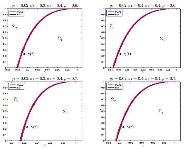
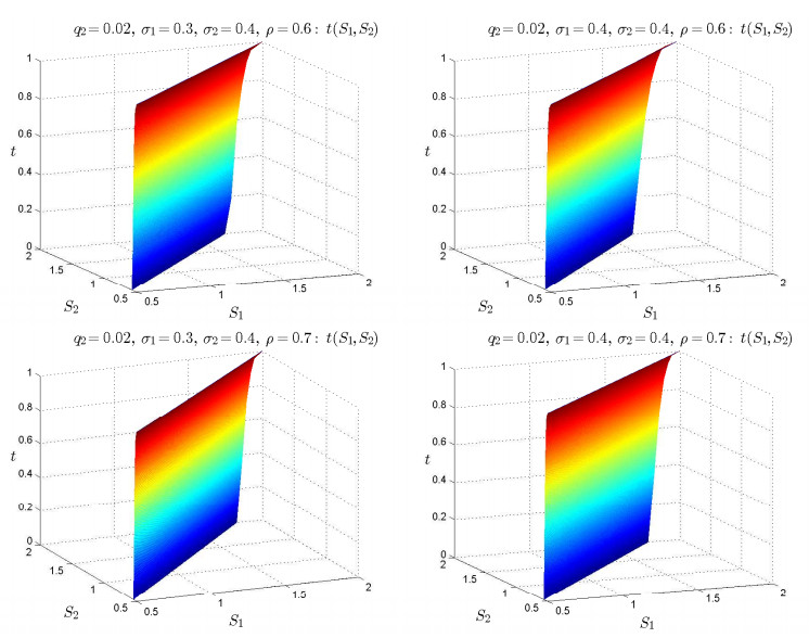
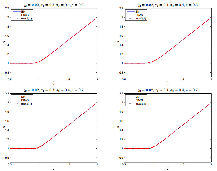
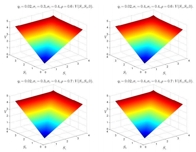
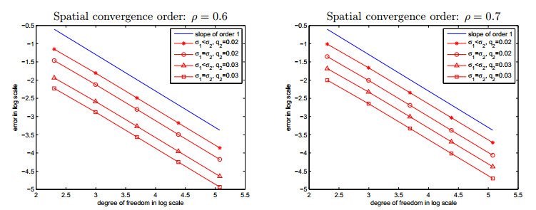
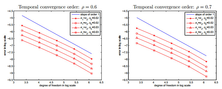
In this paper, an efficient numerical algorithm is proposed for the valuation of unilateral American better-of options with two underlying assets. The pricing model can be described as a backward parabolic variational inequality with variable coefficients on a two-dimensional unbounded domain. It can be transformed into a one-dimensional bounded free boundary problem by some conventional transformations and the far-field truncation technique. With appropriate boundary conditions on the free boundary, a bounded linear complementary problem corresponding to the option pricing is established. Furthermore, the full discretization scheme is obtained by applying the backward Euler method and the finite element method in temporal and spatial directions, respectively. Based on the symmetric positive definite property of the discretized matrix, the value of the option and the free boundary are obtained simultaneously by the primal-dual active-set method. The error estimation is established by the variational theory. Numerical experiments are carried out to verify the efficiency of our method at the end.
- American better-of option,
- far-field truncation technique,
- linear complementary problem,
- finite element method,
- primal-dual active-set method
Citation: Yiyuan Qian, Haiming Song, Xiaoshen Wang, Kai Zhang. Primal-dual active-set method for solving the unilateral pricing problem of American better-of options on two assets[J]. Electronic Research Archive, 2022, 30(1): 90-115. doi: 10.3934/era.2022005

Related Papers:

Abstract

In this paper, an efficient numerical algorithm is proposed for the valuation of unilateral American better-of options with two underlying assets. The pricing model can be described as a backward parabolic variational inequality with variable coefficients on a two-dimensional unbounded domain. It can be transformed into a one-dimensional bounded free boundary problem by some conventional transformations and the far-field truncation technique. With appropriate boundary conditions on the free boundary, a bounded linear complementary problem corresponding to the option pricing is established. Furthermore, the full discretization scheme is obtained by applying the backward Euler method and the finite element method in temporal and spatial directions, respectively. Based on the symmetric positive definite property of the discretized matrix, the value of the option and the free boundary are obtained simultaneously by the primal-dual active-set method. The error estimation is established by the variational theory. Numerical experiments are carried out to verify the efficiency of our method at the end.

References

[1]	X. J. He, W. Chen, A closed-form pricing formula for European options under a new stochastic volatility model with a stochastic long-term mean, Math. Financ. Econ., 15 (2021), 381–396. https://doi.org/10.1007/s11579-020-00281-y doi: 10.1007/s11579-020-00281-y
[2]	X. J. He, S. Lin, A fractional Black-Scholes model with stochastic volatility and European option pricing, Exp. Syst. Appl., 178 (2021), 114983. https://doi.org/10.1016/j.eswa.2021.114983 doi: 10.1016/j.eswa.2021.114983
[3]	S. L. Heston, A closed-form solution for options with stochastic volatility with applications to bond and currency options, Rev. Financ. Stud., 6 (1993), 327–343. https://doi.org/10.1093/rfs/6.2.327 doi: 10.1093/rfs/6.2.327
[4]	R. Caldana, G. Fusai, A general closed-form spread option pricing formula, J. Banking Finance, 37 (2013), 4893–4906. https://doi.org/10.1016/j.jbankfin.2013.08.016 doi: 10.1016/j.jbankfin.2013.08.016
[5]	R. Stulz, Options on the minimum or the maximum of two risky assets: analysis and applications, J. Financ. Econ., 10 (1982), 161–185. https://doi.org/10.1016/0304-405X(82)90011-3 doi: 10.1016/0304-405X(82)90011-3
[6]	L. Jiang, Mathematical modeling and methods of option pricing, World Scientific Publishing Company, 2005. https://doi.org/10.1142/5855
[7]	I. Karatzas, On the pricing of American options, Appl. Math. Optim., 17 (1988), 37–60. https://doi.org/10.1007/BF01448358 doi: 10.1007/BF01448358
[8]	K. S. Tan, K. R. Vetzal, Early exercise regions for exotic options, J. Deriv., 1 (1995), 42–56. https://doi.org/ssrn.com/abstract=6972
[9]	W. K. Wong, K. Xu, Refining the quadratic approximation formula for an American option, Int. J. Theor. Appl. Financ., 4 (2001), 773–781. https://doi.org/10.1142/S0219024901001243 doi: 10.1142/S0219024901001243
[10]	Y. Gao, H. Y. Liu, X. C. Wang, K. Zhang, On an artificial neural network for inverse scattering problems, J. Comput. Phys., 448 (2022), 110771. https://doi.org/10.1016/j.jcp.2021.110771 doi: 10.1016/j.jcp.2021.110771
[11]	M. Broadie, J. Detemple, American option valuation: new bounds, approximations and a comparison of existing methods, Rev. Financ. Stud., 9 (1996), 1211–1250. https://doi.org/10.1093/rfs/9.4.1211 doi: 10.1093/rfs/9.4.1211
[12]	H. Song, Q. Zhang, J. Li, H. Liu, Finite element method for valuation of American lookback options, Math. Numer. Sin., 38 (2016), 245–256. https://doi.org/10.12286/jssx.2016.3.245 doi: 10.12286/jssx.2016.3.245
[13]	J. C. Cox, S. A. Ross, M. Rubinstein, Option pricing: a simplified approach, J. Financ. Econ., 7 (1979), 229–263. https://doi.org/10.1016/0304-405X(79)90015-1 doi: 10.1016/0304-405X(79)90015-1
[14]	K. Amin, A. Khanna, Convergence of American option values from discrete-to continuous-time financial models, Math. Financ., 4 (1994), 289–304. https://doi.org/10.1111/j.1467-9965.1994.tb00059.x doi: 10.1111/j.1467-9965.1994.tb00059.x
[15]	J. A. Tilley, Valuing American options in a path simulation model, Transactions of the Society of Actuaries, 1993. https://doi.org/10.1.1.577.4823
[16]	A. D. Homes, H. Yang, A front-fixing finite element method for the valuation of American options, SIAM J. Sci. Comput., 30 (2008), 2158–2180. https://doi.org/10.1137/070694442 doi: 10.1137/070694442
[17]	Y. Gao, H. Song, X. Wang, K. Zhang, Primal-dual active set method for pricing American better-of option on two assets, Commun. Nonlinear Sci. Numer. Simul., 80 (2020), 104976. https://doi.org/10.1016/j.cnsns.2019.104976 doi: 10.1016/j.cnsns.2019.104976
[18]	X. Pang, H. Song, X. Wang, K. Zhang, An efficient numerical method for the valuation of American better-of options based on the front-fixing transform and the far field truncation, Adv. Appl. Math. Mech., 12 (2020), 902–919. https://doi.org/aamm.OA-2019-0107
[19]	H. Han, X. Wu, A fast numerical method for the Black-Scholes equation of American options, SIAM J. Numer. Anal., 41 (2003), 2081–2095. https://doi.org/10.1137/S0036142901390238 doi: 10.1137/S0036142901390238
[20]	M. Ehrhardt, R. E. Mickens, A fast, stable and accurate numerical method for the Black-Scholes equation of American options, Int. J. Theor. Appl. Financ., 11 (2008), 471–501. https://doi.org/10.1142/S0219024908004890 doi: 10.1142/S0219024908004890
[21]	R. Kangro, R. Nicolaides, Far field boundary conditions for Black-Scholes equations, SIAM J. Numer. Anal., 38 (2000), 1357–1368. https://doi.org/10.1137/S0036142999355921 doi: 10.1137/S0036142999355921
[22]	K. Ito, K. Kunisch, Augmented lagrangian methods for nonsmooth convex optimization in Hilbert spaces, Nonlinear Anal.: Theory, Methods Appl., 41 (2000), 591–616. https://doi.org/10.1016/S0362-546X(98)00299-5 doi: 10.1016/S0362-546X(98)00299-5
[23]	M. Hinterm$\ddot{u}$ller, K. Ito, K. Kunisch, The primal-dual active set strategy as a semi-smooth newton method, SIAM J. Optim., 13 (2002), 865–888. https://doi.org/10.1137/S1052623401383558 doi: 10.1137/S1052623401383558
[24]	M. Bergounioux, K. Ito, K. Kunisch, Primal-dual strategy for constrained optimal control problem, SIAM J. Control Optim., 37 (1999), 1176–1194. https://doi.org/10.1137/S0363012997328609 doi: 10.1137/S0363012997328609
[25]	H. Song, X. Wang, K. Zhang, Q. Zhang, Primal-dual active set method for American lookback put option pricing, East Asian J. Appl. Math., 7 (2017), 603–614. https://doi.org/10.4208/eajam.060317.020617a doi: 10.4208/eajam.060317.020617a
[26]	R. Zhang, H. Song, N. Luan, Weak Galerkin finite element method for valuation of American options, Front. Math. China, 9 (2014), 455–476. https://doi.org/10.1007/s11464-014-0358-6 doi: 10.1007/s11464-014-0358-6
[27]	J. R. Cannon, The one-dimensional heat equation, Cambridge University Press, 1984. https://doi.org/10.1017/CBO9781139086967
[28]	H. Song, Q. Zhang, R. Zhang, A fast numerical method for the valuation of American lookback put options, Commun. Nonlinear Sci. Numer. Simul., 27 (2015), 302–313. https://doi.org/10.1016/j.cnsns.2015.03.010 doi: 10.1016/j.cnsns.2015.03.010
[29]	G. Strang, Approximation in the finite element method, Numer. Math., 19 (1972), 81–98. https://doi.org/10.1007/BF01395933 doi: 10.1007/BF01395933
[30]	C. Johnson, A convergence estimate for an approximation of parabolic variational inequalities, SIAM J. Numer. Anal., 13 (1976), 599–606. https://doi.org/10.1137/0713050 doi: 10.1137/0713050
[31]	A. Antuña, J. Guirao, M. Lópeaz, On the perturbations of maps obeying Shannon-Whittaker-Kotel'nikov's theorem generalization, Adv. Diff. Equations, 1 (2021), 1–12. https://doi.org/10.1186/s13662-021-03535-1 doi: 10.1186/s13662-021-03535-1
[32]	X. J. He, W. Chen, Pricing foreign exchange options under a hybrid Heston-Cox-Ingersoll-Ross model with regime switching, IMA J. Manage. Math., (2021), dpab013. https://doi.org/10.1093/imaman/dpab013
[33]	X. J. He, S. Lin, An analytical approximation formula for barrier option prices under the Heston model, Comput. Econ., (2021). https://doi.org/10.1007/s10614-021-10186-7
[34]	D. Ziane, M. H. Cherif, C. Catteni, K. Belghaba, Yang-Laplace decomposition method for nonlinear system of local fractional partial differential equations, Appl. Math. Nonlinear Sci., 4 (2019), 489–502. https://doi.org/10.2478/AMNS.2019.2.00046 doi: 10.2478/AMNS.2019.2.00046
[35]	Y. Deng, H. Liu, X. Wang, D. Wei, L. Zhu, Simultaneous recovery of surface heat flux and thickness of a solid structure by ultrasonic measurements, Electron. Res. Arch., 29 (2021), 3081–3096. https://doi.org/10.3934/era.2021027. doi: 10.3934/era.2021027
[36]	W. Yin, W. Yang, H. Liu, A neural network scheme for recovering scattering obstacles with limited phaseless far-field data, J. Comput. Phys., 417 (2020), 109594. https://doi.org/10.1016/j.jcp.2020.109594 doi: 10.1016/j.jcp.2020.109594

Reader Comments

Your name:*

Email:*
© 2022 the Author(s), licensee AIMS Press. This is an open access article distributed under the terms of the Creative Commons Attribution License (http://creativecommons.org/licenses/by/4.0)