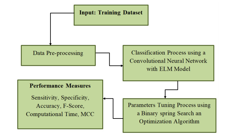
Lockdowns were implemented in nearly all countries in the world in order to reduce the spread of COVID-19. The majority of the production activities like industries, transportation, and construction were restricted completely. This unprecedented stagnation of resident's consumption and industrial production has efficiently reduced air pollution emissions, providing typical and natural test sites to estimate the effects of human activity controlling on air pollution control and reduction. Air pollutants impose higher risks on the health of human beings and also damage the ecosystem. Previous research has used machine learning (ML) and statistical modeling to categorize and predict air pollution. This study developed a binary spring search optimization with hybrid deep learning (BSSO-HDL) for air pollution prediction and an air quality index (AQI) classification process during the pandemic. At the initial stage, the BSSO-HDL model pre-processes the actual air quality data and makes it compatible for further processing. In the presented BSSO-HDL model, an HDL-based air quality prediction and AQI classification model was applied in which the HDL was derived by the use of a convolutional neural network with an extreme learning machine (CNN-ELM) algorithm. To optimally modify the hyperparameter values of the BSSO-HDL model, the BSSO algorithm-based hyperparameter tuning procedure gets executed. The experimental outcome demonstrates the promising prediction classification performance of the BSSO-HDL model. This model, developed on the Python platform, was evaluated using the coefficient of determination R2, the mean absolute error (MAE), and the root mean squared error (RMSE) error measures. With an R2 of 0.922, RMSE of 15.422, and MAE of 10.029, the suggested BSSO-HDL technique outperforms established models such as XGBoost, support vector machines (SVM), random forest (RF), and the ensemble model (EM). This demonstrates its ability in providing precise and reliable AQI predictions.
Citation: Sreenivasulu Kutala, Harshavardhan Awari, Sangeetha Velu, Arun Anthonisamy, Naga Jyothi Bathula, Syed Inthiyaz. Hybrid deep learning-based air pollution prediction and index classification using an optimization algorithm[J]. AIMS Environmental Science, 2024, 11(4): 551-575. doi: 10.3934/environsci.2024027
Lockdowns were implemented in nearly all countries in the world in order to reduce the spread of COVID-19. The majority of the production activities like industries, transportation, and construction were restricted completely. This unprecedented stagnation of resident's consumption and industrial production has efficiently reduced air pollution emissions, providing typical and natural test sites to estimate the effects of human activity controlling on air pollution control and reduction. Air pollutants impose higher risks on the health of human beings and also damage the ecosystem. Previous research has used machine learning (ML) and statistical modeling to categorize and predict air pollution. This study developed a binary spring search optimization with hybrid deep learning (BSSO-HDL) for air pollution prediction and an air quality index (AQI) classification process during the pandemic. At the initial stage, the BSSO-HDL model pre-processes the actual air quality data and makes it compatible for further processing. In the presented BSSO-HDL model, an HDL-based air quality prediction and AQI classification model was applied in which the HDL was derived by the use of a convolutional neural network with an extreme learning machine (CNN-ELM) algorithm. To optimally modify the hyperparameter values of the BSSO-HDL model, the BSSO algorithm-based hyperparameter tuning procedure gets executed. The experimental outcome demonstrates the promising prediction classification performance of the BSSO-HDL model. This model, developed on the Python platform, was evaluated using the coefficient of determination R2, the mean absolute error (MAE), and the root mean squared error (RMSE) error measures. With an R2 of 0.922, RMSE of 15.422, and MAE of 10.029, the suggested BSSO-HDL technique outperforms established models such as XGBoost, support vector machines (SVM), random forest (RF), and the ensemble model (EM). This demonstrates its ability in providing precise and reliable AQI predictions.

| [1] |
Rahman M M, Paul K C, Hossain M A, et al. (2021) Machine Learning on the COVID-19 Pandemic, Human Mobility and Air Quality: A Review. IEEE Access 9: 72420–72450. https://doi.org/10.1109/ACCESS.2021.3079121 doi: 10.1109/ACCESS.2021.3079121

|
| [2] |
Xing X, Xiong Y, Yang R, et al. (2021) Predicting the effect of confinement on the COVID-19 spread using machine learning enriched with satellite air pollution observations. Proc Natl Acad Sci 118: 33. https://doi.org/10.1073/pnas.2109098118 doi: 10.1073/pnas.2109098118
|
| [3] |
Sethi J K, Mittal M (2020) Monitoring the Impact of Air Quality on the COVID-19 Fatalities in Delhi, India: Using Machine Learning Techniques. Disaster Med Public Health Prep 6: 604-611. https://doi.org/10.1017/dmp.2020.372 doi: 10.1017/dmp.2020.372
|
| [4] |
Yang J, Wen Y, Wang Y, et al. (2021) From COVID-19 to future electrification: Assessing traffic impacts on air quality by a machine-learning model. P Nati A Sci 118: e2102705118. https://doi.org/10.1073/pnas.2102705118 doi: 10.1073/pnas.2102705118
|
| [5] |
Rybarczyk Y, Zalakeviciute R (2021) Assessing the COVID‐19 Impact on Air Quality: A Machine Learning Approach. Geophysl Res Lett 48: e2020GL091202. https://doi.org/10.1029/2020GL091202 doi: 10.1029/2020GL091202
|
| [6] |
Liu H, Yue F, Xie Z (2022) Quantify the role of anthropogenic emission and meteorology on air pollution using machine learning approach: A case study of PM2.5 during the COVID-19 outbreak in Hubei Province, China. Environ Pollut 300: 118932. https://doi.org/10.1016/j.envpol.2022.118932 doi: 10.1016/j.envpol.2022.118932
|
| [7] |
Gatti R C, Velichevskaya A, Tateo A, et al. (2020) Machine learning reveals that prolonged exposure to air pollution is associated with SARS-CoV-2 mortality and infectivity in Italy. Environ Pollut 267: 115471. https://doi.org/10.1016/j.envpol.2020.115471 doi: 10.1016/j.envpol.2020.115471
|
| [8] |
Gao M, Yang H, Xiao Q, et al. (2022) COVID-19 lockdowns and air quality: Evidence from grey spatiotemporal forecasts. Socio-Econ Plan Sci 83: 101228. https://doi.org/10.1016/j.seps.2022.101228 doi: 10.1016/j.seps.2022.101228
|
| [9] |
Wijnands J S, Nice K A, Seneviratne S, et al. (2022) The impact of the COVID-19 pandemic on air pollution: A global assessment using machine learning techniques. Atmos Pollut Res 13: 101438. https://doi.org/10.1016/j.apr.2022.101438 doi: 10.1016/j.apr.2022.101438
|
| [10] |
Wibowo F W (2021) Prediction of air quality in Jakarta during the COVID-19 outbreak using long short-term memory machine learning. IOP Conference Series: Earth and Environmental Science 704: 012046. https://doi.org/10.1088/1755-1315/704/1/012046 doi: 10.1088/1755-1315/704/1/012046
|
| [11] |
Stephan T, Al-Turjman F, Ravishankar M, et al. (2022) Machine learning analysis on the impacts of COVID-19 on India's renewable energy transitions and air quality. Environ Sci Pollut Res 29: 79443–79465. doi: 10.1007/s11356-022-20997-2. https://doi.org/10.1007/s11356-022-20997-2 doi: 10.1007/s11356-022-20997-2
|
| [12] |
Li G, Tang Y, Yang H (2022) A new hybrid prediction model of air quality index based on secondary decomposition and improved kernel extreme learning machine. Chemosphere 305: 135348. https://doi.org/10.1016/j.chemosphere.2022.135348 doi: 10.1016/j.chemosphere.2022.135348
|
| [13] |
Yang H, Zhang Y, Li G (2023) Air quality index prediction using a new hybrid model considering multiple influencing factors: A case study in China. Atmos Pollut Res 14: 1016777. https://doi.org/10.1016/j.apr.2023.101677 doi: 10.1016/j.apr.2023.101677
|
| [14] | Sassi M S H, Fourati L C (2021) Deep Learning and Augmented Reality for IoT-based Air Quality Monitoring and Prediction System. IEEE 2021. https://doi.org/10.1109/ISNCC52172.2021.9615639 |
| [15] |
Shahne M Z, Sezavar A, Najibi F (2022) A hybrid deep learning model to forecast air quality data based on COVID-19 outbreak in Mashhad, Iran. Ann Civ Environ Eng 6: 019–025. https://doi.org/10.29328/journal.acee.1001035 doi: 10.29328/journal.acee.1001035
|
| [16] |
Tsan Y T, Kristiani E, Liu P Y, et al. (2022) In the Seeking of Association between Air Pollutant and COVID-19 Confirmed Cases Using Deep Learning. Int J Environl Res Pub He 19: 6373. https://doi.org/10.3390/ijerph19116373 doi: 10.3390/ijerph19116373
|
| [17] |
Lovrić M, Pavlović K, Vuković M, et al. (2021) Understanding the true effects of the COVID-19 lockdown on air pollution by means of machine learning. Environ Pollut 274: 115900. https://doi.org/10.1016/j.envpol.2020.115900 doi: 10.1016/j.envpol.2020.115900
|
| [18] |
Tyagi A, Gaur L, Singh G, et al. (2022) Air Quality Index (AQI) Using Time Series Modelling During COVID Pandemic. Lect Notes Electr Eng 2022: 441–452. https://doi.org/10.1007/978-981-16-8546-0_36 doi: 10.1007/978-981-16-8546-0_36
|
| [19] |
Maltare N N, Vahora S (2023) Air quality index prediction using machine learning for Ahmedabad city. Digital. Chemical. Engineering 7: 100093. https://doi.org/10.1016/j.dche.2023.100093 doi: 10.1016/j.dche.2023.100093
|
| [20] |
Xu J, Wang S, Ying N, et al. (2023) Dynamic graph neural network with adaptive edge attributes for air quality prediction: A case study in China. Heliyon 9: 17746. https://doi.org/10.1016/j.heliyon.2023.e17746 doi: 10.1016/j.heliyon.2023.e17746
|
| [21] |
Ghoneim A, Muhammad G, Hossain M S (2020) Cervical cancer classification using convolutional neural networks and extreme learning machines. Future Gener Comp Sy 102: 643–649. https://doi.org/10.1016/j.future.2019.09.015 doi: 10.1016/j.future.2019.09.015
|
| [22] |
Dehghani M, Montazeri Z, Dehghani A, et al. (2021) Binary Spring Search Algorithm for Solving Various Optimization Problems. Appl Sci 11: 1286. https://doi.org/10.3390/app11031286 doi: 10.3390/app11031286
|
| [23] |
Kamalraj R, Neelakandan S, Kumar M R, et al. (2021) Interpretable filter based convolutional neural network (IF-CNN) for glucose prediction and classification using PD-SS algorithm. Measurement 183: 109804. https://doi.org/10.1016/j.measurement.2021.109804 doi: 10.1016/j.measurement.2021.109804
|
| [24] |
Kavitha T, Mathai P P, Karthikeyan C, et al. (2021) Deep Learning Based Capsule Neural Network Model for Breast Cancer Diagnosis Using Mammogram Images. Interdiscip Sci 2021: 1-17. https://doi.org/10.1007/s12539-021-00467-y doi: 10.1007/s12539-021-00467-y
|
| [25] |
Reshma G, Al-Atroshi C, Nassa V K, et al. (2022) Deep Learning-Based Skin Lesion Diagnosis Model Using Dermoscopic Images. Intell Autom Soft Co 31: 621–634. https://doi.org/10.32604/iasc.2022.019117 doi: 10.32604/iasc.2022.019117
|
| [26] |
Harshavardhan A, Boyapati P, Neelakandan S, et al. (2022) LSGDM with Biogeography-Based Optimization (BBO) Model for Healthcare Applications. J Healthc Eng 2022: 1–11. https://doi.org/10.1155/2022/2170839 doi: 10.1155/2022/2170839
|
| [27] |
Neelakandan S, Beulah J R, Prathiba L, et al. (2022) Blockchain with deep learning-enabled secure healthcare data transmission and diagnostic model. Int J Model Simul Sc 13: 2241006. https://doi.org/10.1142/S1793962322410069 doi: 10.1142/S1793962322410069
|
| [28] |
Mao W, Wang W, Jiao L, et al. (2020) Modeling air quality prediction using a deep learning approach: Method optimization and evaluation. Sustain Cities Soc 65: 102567. https://doi.org/10.1016/j.scs.2020.102567 doi: 10.1016/j.scs.2020.102567
|
| [29] |
Jurado X, Reiminger N, Benmoussa M, et al. (2022). Deep learning methods evaluation to predict air quality based on Computational Fluid Dynamics. Expert System Applications 203: 117294. https://doi.org/10.1016/j.eswa.2022.117294 doi: 10.1016/j.eswa.2022.117294
|


Figures(15) / Tables(7)

Sreenivasulu Kutala, Harshavardhan Awari, Sangeetha Velu, Arun Anthonisamy, Naga Jyothi Bathula, Syed Inthiyaz. Hybrid deep learning-based air pollution prediction and index classification using an optimization algorithm[J]. AIMS Environmental Science, 2024, 11(4): 551-575. doi: 10.3934/environsci.2024027


 DownLoad: