Hydro-meteorological drought in Addis Ababa: A characterization study

Zinabu A. Alemu; Emmanuel C. Dioha; Michael O. Dioha; Zinabu A. Alemu; Emmanuel C. Dioha; Michael O. Dioha

doi:10.3934/environsci.2021011

AIMS Environmental Science

2021, Volume 8, Issue 2: 148-168. doi: 10.3934/environsci.2021011

Previous Article Next Article

Research article

Hydro-meteorological drought in Addis Ababa: A characterization study

1.
Department of Environmental Health, Ethiopian Public Health Institute, P.O.Box: 1242, Addis Ababa, Ethiopia
2.
Department of Geology, Federal University of Technology Owerri, P.M.B. 1526, Owerri Imo State, Nigeria
3.
Department of Energy and Environment, TERI School of Advanced Studies, 10 Institutional Area, Vasant Kunj, New Delhi-110 070, India

Received: 28 December 2020 Accepted: 05 April 2021 Published: 20 April 2021

Drought is one of the most natural hazards that cause damage to ecosystems, agricultural production, and water resources. This study has analyzed seasonal and annual rainfall trends using monthly data series of 33 years (1983–2015) in Addis Ababa city over three stations namely; Sendafa, Bole, and Observation. Here, we examined the occurrence of historical drought trends in the study jurisdiction. The Reconnaissance Drought Index (RDI) and the Standardized Precipitation Index (SPI) were employed to find long-term drought trends as well as to examine the occurrence of drought history at a longer duration. The analysis indicated that severe drought conditions were observed for SPI and RDI indices in the year 2013 for Bole station, while medium droughts were recorded for the years 1991 and 2002 for all stations. Similarly, the RDI indices for 1996 was recorded as severe drought for the Observatory station. On the other hand, higher variability (coefficient of variation) of rainfall during winter seasons were 95.8%, 95.9%, and 77.9% for Sendafa, Bole, and Observatory stations respectively. However, the lower coefficient of variation during annual rainfall was 15.59% for Sendafa, 14.38% for Bole, and 13.98% for the Observatory station. Furthermore, the drought severity classification for the long-term drought analysis of annual precipitation shows that 3% of severe drought, 12% of moderate drought, and 85% of the normal condition were recorded in Bole station. The severe and moderate drought indices due to the reduction of rainfall, temperature change, and other factors can cause a shortage of urban water supply. Thus, the results of this study will help the water sector professionals in forecasting weather variations and for better management of urban water resources.
- rainfall,
- standard precipitation index,
- drought,
- reconnaissance drought index,
- DrinC software,
- Addis Ababa
Citation: Zinabu A. Alemu, Emmanuel C. Dioha, Michael O. Dioha. Hydro-meteorological drought in Addis Ababa: A characterization study[J]. AIMS Environmental Science, 2021, 8(2): 148-168. doi: 10.3934/environsci.2021011

Related Papers:

Abstract

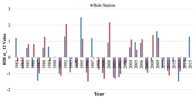
Drought is one of the most natural hazards that cause damage to ecosystems, agricultural production, and water resources. This study has analyzed seasonal and annual rainfall trends using monthly data series of 33 years (1983–2015) in Addis Ababa city over three stations namely; Sendafa, Bole, and Observation. Here, we examined the occurrence of historical drought trends in the study jurisdiction. The Reconnaissance Drought Index (RDI) and the Standardized Precipitation Index (SPI) were employed to find long-term drought trends as well as to examine the occurrence of drought history at a longer duration. The analysis indicated that severe drought conditions were observed for SPI and RDI indices in the year 2013 for Bole station, while medium droughts were recorded for the years 1991 and 2002 for all stations. Similarly, the RDI indices for 1996 was recorded as severe drought for the Observatory station. On the other hand, higher variability (coefficient of variation) of rainfall during winter seasons were 95.8%, 95.9%, and 77.9% for Sendafa, Bole, and Observatory stations respectively. However, the lower coefficient of variation during annual rainfall was 15.59% for Sendafa, 14.38% for Bole, and 13.98% for the Observatory station. Furthermore, the drought severity classification for the long-term drought analysis of annual precipitation shows that 3% of severe drought, 12% of moderate drought, and 85% of the normal condition were recorded in Bole station. The severe and moderate drought indices due to the reduction of rainfall, temperature change, and other factors can cause a shortage of urban water supply. Thus, the results of this study will help the water sector professionals in forecasting weather variations and for better management of urban water resources.

References

[1]	Najihah TS, Ibrahim M H, Zain NAM, et al. (2020) Activity of the oil palm seedlings exposed to a different rate of potassium fertilizer under water stress condition. AIMS Environ Sci 7: 46-68. doi: 10.3934/environsci.2020004
[2]	Sönmez FK, Kömüscü AÜ, Erkan A, et al. (2005) An analysis of spatial and temporal dimension of drought vulnerability in Turkey using the standardized precipitation index. Nat Hazards 35: 243-264. doi: 10.1007/s11069-004-5704-7
[3]	Manjowe M, Mushore TD, Gwenzi J, et al. (2018) Circulation mechanisms responsible for wet or dry summers over Zimbabwe. AIMS Environ Sci 5: 154-172. doi: 10.3934/environsci.2018.3.154
[4]	Smakhtin VU, Hughes DA, (2007) Automated estimation and analyses of meteorological drought characteristics from monthly rainfall data. Environ Modell Softw 22: 880-890. doi: 10.1016/j.envsoft.2006.05.013
[5]	Christy JR (2019) Examination of extreme rainfall events in two regions of the United States since the 19th century. AIMS Environ Sci 6: 109-126. doi: 10.3934/environsci.2019.2.109
[6]	Yahaya I, Adamu SJ, Muhammed BB, (2017) The use of Standardized Precipitation Index (SPI) for Drought Intensity Assessment in North-Eastern Nigeria. Researchjournal's J Geo 4:1-13
[7]	Feyissa G, Zeleke G, Bewket W, et al. (2018) Downscaling of future temperature and precipitation extremes in Addis Ababa under climate change. Climate 6: 58. doi: 10.3390/cli6030058
[8]	Engida M (1999) Annual rainfall and evapotranspiration in Ethiopia. Ethiopian Journal of Natural Resources 1: 137-154.
[9]	IPCC (2007) Climate Change 2007: Impacts, Adaptation and Vulnerability. Contribution of Working Group Ⅱ to the Fourth Assessment Report of the Intergovernmental Panel on Climate Change. Edited by Parry, M., Canziani, O., Palutikof, J., Linden, P.vd., Hanson, C., Cambridge University Press 32 Avenue of the Americas, New York, USA, 10013-2473.
[10]	Alemu ZA, Dioha MO, (2020a) Climate change and trend analysis of temperature: the case of Addis Ababa, Ethiopia. Environ Syst Res 9: 1-15.
[11]	FDRE, Ethiopian Government Portal, 2018. Available from: http://www.ethiopia.gov.et/addis-ababa-city-administration.
[12]	Niemeyer S, New drought indices. European Commission, DG Joint Research Centre, Institute for Environment and Sustainability, T.P. 261, JRC-IES, I-21020 Ispra (VA), Italy, 2020 Availablefrom: https://om.ciheam.org/om/pdf/a80/00800451.pdf
[13]	Gebreyesus M, Cherint A, Ashine T, et al. Drought Analysis Using Reconnaissance Drought Index (RDI): In the case of Awash River Basin, Ethiopia2020. Available from: https://www.researchgate.net/publication/344440865_Drought_analysis_using_reconnaissance_drought_index_RDI_In_the_case_of_Awash_River_Basin_Ethiopia
[14]	Tigkas D, Vangelis H, Tsakiris G (2013) The RDI as a composite climatic index. E.W. Publications. European Water 41: 17-22.
[15]	McKee TB, Doesken NJ, Kleist J (1993) The relationship of drought frequency and duration of time scales. Eighth Conference on Applied Climatology, American Meteorological Society, Anaheim CA.
[16]	Aksoy H, Onoz B, Cetin M, et al. (2018) SPI-based Drought Severity-Duration-Frequency Analysis. 13th International Congress on Advances in Civil Engineering, Izmir/Turkey.
[17]	Pashiardis S, Michaelides S (2008) Implementation of the Standardized Precipitation Index (SPI) and the Reconnaissance Drought Index (RDI) for Regional Drought Assessment: A case study for Cyprus. E.W. Publications. Eur Water 23/24: 57-65.
[18]	Asadi-Zarch MA, Malekinezhad H, Mobin MH, et al. (2011) Drought Monitoring by Reconnaissance Drought Index (RDI) in Iran. Water Resour Manag 25: 3485-3504. doi: 10.1007/s11269-011-9867-1
[19]	Ansarifard S, Shamsnia SA (2018) Monitoring drought by Reconnaissance Drought Index (RDI) and Standardized Precipitation Index (SPI) using DrinC software. Water Utility J 20: 29-35.
[20]	Hayes MJ, Svoboda MD, Wilhite DA, et al. (1999) Monitoring the 1996 Drought Using the Standardized Precipitation Index. B Am Meteorol Soc 80: 429-438. doi: 10.1175/1520-0477(1999)080<0429:MTDUTS>2.0.CO;2
[21]	Zarei AR, Moghimi MM, Mahmoudi MR (2016) Analysis of Changes in Spatial Pattern of Drought Using RDI Index in south of Iran. Water Resour Manag 30: 3723-3743. doi: 10.1007/s11269-016-1380-0
[22]	Pramudya Y, Onishi T, (2018) Assessment of the Standardized Precipitation Index (SPI) in Tegal City, Central Java, Indonesia. IOP Conf. Series: Earth Environ Sci 129: 012-019.
[23]	Maroua BA, Nouiri I, (2018) Study of trends in historical variation and mapping of drought events in Tunisia: A global assessment of Standardized precipitation index (SPI) and Reconnaissance drought index (RDI) for the period 1973-2016. 3^rd International Conference on Integrated Environmental Management for Sustainable Development. ISSN 1737-3638.
[24]	Vangelis H, Tigkas D, Tsakiris G, (2012) The effect of PET method on Reconnaissance Drought Index (RDI) calculation. J Arid Environ 88: 130-140. doi: 10.1016/j.jaridenv.2012.07.020
[25]	Tsakiris G, Vangelis H, Pangalou D, (2007) Regional Drought Assessment Based on the Reconnaissance Drought Index (RDI). Water Resour Manage 21: 821-833. doi: 10.1007/s11269-006-9105-4
[26]	Fitsume Y, (2014) Precipitation Extremes and their Pattern in the Central Highlands of Ethiopia: SPI Based Analysis. J Nat Sci Res 4: 92-97.
[27]	Gidey E, Dikinya O, Sebego R, et al. (2018) Modeling the Spatio-Temporal Meteorological Drought Characteristics Using the Standardized Precipitation Index (SPI) in Raya and Its Environs, Northern Ethiopia. Earth Sys Environ 2: 281-292. doi: 10.1007/s41748-018-0057-7
[28]	Spinoni J, Naumann G, Carrao H, et al. (2013) World drought frequency, duration, and severity for 1951-2010. Int J Climatol 34: 2792-2804. doi: 10.1002/joc.3875
[29]	Tigkas D, Vangelis H, Tsakiris G (2015) DrinC: a software for drought analysis based on drought indices. Earth Sci Inform 8: 697-709. doi: 10.1007/s12145-014-0178-y
[30]	Climate-Ethiopia, Climates to travel world climate guide, 2021. Available from: https://www.climatestotravel.com/climate/ethiopia.
[31]	Alemu ZA, Dioha MO (2020b) Modelling scenarios for sustainable water supply and demand in Addis Ababa city, Ethiopia. Environ Syst Res 9: 1-14.
[32]	FDRE, City Map of Addis Ababa City Administration, Ethiopia, 2020. Available from: http://www.addisababa.gov.et/de/web/guest/city-map
[33]	Rossi G, Bonaccorso B, Vega T (2007) Methods and tools for drought analysis and management, Springer Science and Business Media, Berlin. vol 62. ISBN 978-1-4020-5923-0
[34]	Tsakiris G, Nalbantis I, Pangalou D, et al. (2008) Drought meteorological monitoring network design for the reconnaissance drought index (RDI). In: Franco Lopez A. (Ed.), Proceedings of the 1st International Conference "Drought Management: scientific and technological innovations". Zaragoza, Spain: Option Méditerranéennes, Series A, 80: 57-62.
[35]	Vangelis H, Tigkas D, Tsakiris G (2013) The effect of PET method on Reconnaissance Drought Index (RDI) calculation. J Arid Environ 88: 130-140. doi: 10.1016/j.jaridenv.2012.07.020
[36]	Allen RG, Pereira LS, Raes D, et al. (1998) Crop evapotranspiration: guidelines for computing crop water requirements. FAO irrigation and drainage paper 56, 1^st edition. Rome, Italy.
[37]	Hargreaves GH, Samani ZA (1985) Reference crop evapotranspiration from temperature. Appl Eng Agric 1: 96-99. doi: 10.13031/2013.26773
[38]	Tigkas D (2008) Drought Characterization and Monitoring in Regions of Greece. Eur Water 23/24: 29-39.
[39]	Khanmohammadi N, Rezaie H, Montaseri M, et al. (2017) The Effect of Temperature Adjustment on Reference Evapotranspiration and Reconnaissance Drought Index (RDI) in Iran. Water Resour Manag 31: 5001-5017. doi: 10.1007/s11269-017-1793-4
[40]	Gupta SP (2007) Statistical Methods. Seventh Revised and Enlarged Edition ed. Sultan Chand and Sons, Educational Publisher. New Delhi.
[41]	Helsel DR, Hirsch RM (2002) Statistical methods in water resources. Techniques of water-resources investigations of the United States geological survey, book 4, hydrologic analysis and interpretation. U. S. Geological survey
[42]	Philip S, Kew SF, Oldenborgh GJ, et al. (2018) Attribution Analysis of the Ethiopian Drought of 2015. American Meteorological Society 2465-2486.
[43]	Jamshidi H, Khalili D, Zadeh MR, et al. (2011) Assessment and comparison of SPI and RDI meteorological drought indices in selected synoptic stations of Iran. In World Environmental and Water Resources Congress 2011: Bearing Knowledge for Sustainability, 1161-1173.
[44]	Haied N, Foufou A, Chaab S, et al. (2017) Drought assessment and monitoring using meteorological indices in a semi-arid region. Energy Procedia 119: 518-529. doi: 10.1016/j.egypro.2017.07.064
[45]	Shah R, Bharadiya N, Manekar V (2015) Drought index computation using Standardized Precipitation Index (SPI) method for Surat district, Gujarat. J Aquat Proced 4: 1243-1249. doi: 10.1016/j.aqpro.2015.02.162
[46]	Thilakarathne M, Sridhar V (2017) Characterization of future drought conditions in the Lower Mekong River Basin. Weather Climate Extremes 17: 47-58. doi: 10.1016/j.wace.2017.07.004
[47]	Khatiwada KR, Pandey VP (2019) Characterization of hydro-meteorological drought in Nepal Himalaya: A case of Karnali River Basin. Weather Climate Extremes 26: 100239. doi: 10.1016/j.wace.2019.100239
[48]	Abdelmalek MB, Nouiri I (2020) Study of trends and mapping of drought events in Tunisia and their impacts on agricultural production. Sci Total Environ 734: 139311. doi: 10.1016/j.scitotenv.2020.139311
[49]	Almedeij J, (2014) Drought analysis for kuwait using standardized precipitation index. The Sc World J. 2014
[50]	NMSA, (1996) Climatic and agro climatic resources of Ethiopia. National Meteorology Service Agency of Ethiopia, Addis Ababa. 1: 137.
[51]	Temam D, Uddameri V, Mohammadi G, et al. (2019) Long-Term Drought Trends in Ethiopia with Implications for Dryland Agriculture. MDPI-Water 11: 2571. doi: 10.3390/w11122571
[52]	Cermak V, Bodri L, Safanda J, et al. (2019) Variability trends in the daily air temperatures series Running head: Variability trends prague. AIMS Environ Sci 6: 167-185. doi: 10.3934/environsci.2019.3.167

Reader Comments

Your name:*

Email:*
© 2021 the Author(s), licensee AIMS Press. This is an open access article distributed under the terms of the Creative Commons Attribution License (http://creativecommons.org/licenses/by/4.0)