Citation: Dong Chen, Marcus Thatcher, Xiaoming Wang, Guy Barnett, Anthony Kachenko, Robert Prince. Summer cooling potential of urban vegetation—a modeling study for Melbourne, Australia[J]. AIMS Environmental Science, 2015, 2(3): 648-667. doi: 10.3934/environsci.2015.3.648
| [1] | Alejandra S. Coronel, Susana R. Feldman, Emliano Jozami, Kehoe Facundo, Rubén D. Piacentini, Marielle Dubbeling, Francisco J. Escobedo . Effects of urban green areas on air temperature in a medium-sized Argentinian city. AIMS Environmental Science, 2015, 2(3): 803-826. doi: 10.3934/environsci.2015.3.803 |
| [2] | Mary Thornbush . Urban greening for low carbon cities—introduction to the special issue. AIMS Environmental Science, 2016, 3(1): 133-139. doi: 10.3934/environsci.2016.1.133 |
| [3] | Mary Thornbush . Urban agriculture in the transition to low carbon cities through urban greening. AIMS Environmental Science, 2015, 2(3): 852-867. doi: 10.3934/environsci.2015.3.852 |
| [4] | Jian Zhang, Zhonghua Gou, Leigh Shutter . Effects of internal and external planning factors on park cooling intensity: field measurement of urban parks in Gold Coast, Australia. AIMS Environmental Science, 2019, 6(6): 417-434. doi: 10.3934/environsci.2019.6.417 |
| [5] | Alessio Russo, Francisco J Escobedo, Stefan Zerbe . Quantifying the local-scale ecosystem services provided by urban treed streetscapes in Bolzano, Italy. AIMS Environmental Science, 2016, 3(1): 58-76. doi: 10.3934/environsci.2016.1.58 |
| [6] | Lin Ma, Jun Zhang, Lixing Chen, Shuling Xiao, Yingzi Zhang . A field research on the impact of underlying surface configuration on street thermal environment in Lhasa. AIMS Environmental Science, 2019, 6(6): 483-503. doi: 10.3934/environsci.2019.6.483 |
| [7] | Beth Ravit, Frank Gallagher, James Doolittle, Richard Shaw, Edwin Muñiz, Richard Alomar, Wolfram Hoefer, Joe Berg, Terry Doss . Urban wetlands: restoration or designed rehabilitation?. AIMS Environmental Science, 2017, 4(3): 458-483. doi: 10.3934/environsci.2017.3.458 |
| [8] | Kumari Anjali, YSC Khuman, Jaswant Sokhi . A Review of the interrelations of terrestrial carbon sequestration and urban forests. AIMS Environmental Science, 2020, 7(6): 464-485. doi: 10.3934/environsci.2020030 |
| [9] | Huixuan Li, Cuizhen Wang, Yuqin Jiang, Andrew Hug, Yingru Li . Spatial assessment of sewage discharge with urbanization in 2004–2014, Beijing, China. AIMS Environmental Science, 2016, 3(4): 842-857. doi: 10.3934/environsci.2016.4.842 |
| [10] | Dominic Bowd, Campbell McKay, Wendy S. Shaw . Urban greening: environmentalism or marketable aesthetics. AIMS Environmental Science, 2015, 2(4): 935-949. doi: 10.3934/environsci.2015.4.935 |
Over 50% of the world’s population lives in cities with much higher urbanization levels in developed countries [1]. In Australia, the percentage of urban population of 86% has only increased slightly from several decades ago; however, the total Australian population has doubled in the past 50 years [2]. The rapid urbanization has transformed some vegetated lands into urban areas with engineered infrastructure accompanied by increased heat generation from anthropogenic activities and heat absorption and storage. Such heat generation, heat absorption and storage combined with slow heat dispersion result in the urban heat island (UHI) effect. Several studies have reported a mean UHI effect of around 1 to 2 °C in Melbourne, Victoria, Australia which has gradually increased at a rate of approximately 0.2 °C per decade from 1958 to 2007 [3,4]. This rate of increase in the UHI effect is in similar range as that reported by Wu and Yang [5] for the Yangtze River Delta city cluster region in China. Without effective interference, the UHI effect in Melbourne is likely to continue, if not further increase considering that the existing Melbourne metropolitan blue print relies heavily on the further development in established urban areas in order to maintain sustainable and manageable metropolitan service infrastructure [6].
When coupled with summer heat waves, the UHI effect can pose significant threats to the urban environment due to increased pollution levels, heat stress, excess energy consumption and impact on other service infrastructure [7,8,9] and human health[10,11,12,13,14,15,16]. The heat wave event in Melbourne during the summer of 2009 may have resulted in 374 excess deaths over what would normally be expected for the period. This reflects in a 62% increase in total all-cause mortality for that period-[17]. The relationship between heat and mortality has long been recognized [11]. Nicholls et al. [14] analyzed the mortality rate in Melbourne from 1979 to 2001 and reported that excess heat related mortality amongst the population aged over 65 may increase rapidly when the daily mean temperatures (the average of yesterday’s maximum and this morning’s minimum) exceeds 30 °C.
The situation of urban summer heat stress is likely to be further exacerbated in Australia by global warming considering the projected increase in the number of warm nights, heat wave frequency and duration [18]. The summer heat driven by the increasing UHI effect and heat wave frequency/intensity caused by urbanization and global warming presents significant environmental and social challenges for governments and communities around the world [5,13,19,20,21,22]. Many countries have integrated climate change mitigation and adaptation into policy frameworks such as policies to accelerate investment in energy efficiency, renewable energy and other greenhouse gas (GHG) emission reduction technologies [23,24,25]. Implementing urban greening and cool surfaces have attracted substantial research and community interests and show promise in mitigating the UHI effect [13,26,27,28,29,30]. Urban greening can mitigate the UHI effect by promoting tree planting to shade buildings and to cool the ambient by evapotranspiration of vegetation [31,32,33,34]. Cool surfaces can mitigate the UHI effect by using reflective roofs and paving surfaces to reduce the heat absorption. Urban greening and cool surfaces can reduce the cooling energy demand and thus GHG emissions in cities [27,35,36,37,38].
Using a mesoscale urban climate model, Liu and Bass [31] simulated the local climate of the City of Toronto for 2 days in June 2001 by replacing 50% of building foot print with grassland to represent a 50% green roof coverage scenario. Simulation results showed that Toronto could be 0.1‒0.8 °C cooler as a result of 50% green roof coverage as compared with the base scenario without green roofs. In a similar study, Rosenzweig et al. [32] simulated the impact of nine different levels of urban greening and cool roof coverage scenarios during the summer of 2002 in New York City. They illustrated that urban greening and cool roofs can result in up to 1 °C reduction in the average ambient temperature. Susca et al. [35] monitored the UHI in four areas of New York City from October 2008 through to May 2009 and reported an average of 2 °C difference in temperatures between the most and the least vegetated areas.
Sailor [39] simulated the local urban climate of Los Angeles in response to increased vegetation coverage and showed temperature depression of around 0.8°C. Taha et al. [40] simulated 2 days in a summer of the California’s South Coast Air Basin area and suggested an average 1.0°C cooling effect was achievable with a high vegetation scenario. In the Tel-Aviv urban complex during the period July-August 1996, Shashua-Bar and Hoffman [41] found that the average cooling effect across 11 wooded sites was 2.8 °C.
Using multiple linear regression analysis for satellite imagery land surface temperatures, Kong et al. [42] showed that proper management and planning of green spaces in cities are important in order to reduce UHI impact. Perini and Magliocco [43] quantified the effects of various vegetation scenarios in mitigating summer temperatures with a microclimate model in three Mediterranean cities and showed that for most of the cases examined, vegetation has higher cooling effects in taller building areas. Chen et al. [44] demonstrated the cooling effects of greening in a northern Chinese city, Tianjin, both numerically and using real measurements. They pointed out that the cooling effects by urban greening have a certain limit.
More recently, by carrying out simulations for a Chinese city, Suzhou, using an urban canopy model, Yang et al. [45] reported that both tree planting and grass surfacing are beneficial in cooling the ambient air temperature with tree planting to be generally more effective. Yang et al. [45] found that the daily mean air temperature can be reduced by 1 °C during the simulated summer period with 40% tree coverage. Similarly, using computational fluid dynamics simulations for the city center of Arnhem, the Netherlands, Gromke et al. [46] reported that among different vegetation measures, the strongest cooling by a single vegetative measure was obtained with the avenue-trees with mean and maximum temperature reductions at pedestrian level of 0.43 and 1.6 °C, respectively. They noticed that cooling effective overall resembled a linear superposition of various vegetative measures and that a maximum of 2.0 °C temperature reduction can be obtained with a combination of vegetative measures. Simulations by Middel et al. [47] using a microclimate model for the City of Phoenix, Arizona found that an increase in the tree canopy cover from 10 to 25% can result in an average daytime cooling benefit of up to 2.0 °C in residential neighborhoods.
From these studies it appears that the cooling effect of urban vegetation depends on the specific location due to the variation in the geophysical conditions, urban land usage and vegetation coverage. Furthermore, previous studies are limited to the cooling effects of urban vegetation for the present day (current) climate. The current study investigated the potential of various urban vegetation schemes in mitigating summer temperatures in Melbourne for both current and future climates.
A recently developed urban climate model UCM (urban canopy model)-TAPM (The Air Pollution Model) [48] was used for investigating the impact of various vegetation schemes on the local urban climate in Melbourne. The UCM-TAPM is a computer-based prognostic meteorological model which combines an urban canopy model with a meso-scale climate model TAPM [49].
The UCM is based on the Town Energy Budget approach by Masson [50] and modified to better represent the climates of Australian cities. Figure 1 is a simplified description of the UCM. Shaded areas indicate roofs, walls, roads and vegetation that are represented as energy budgets. Thin solid arrows describe turbulent sensible and latent heat exchanges within the canyon and between the above atmosphere and the below urban area. Thin dashed arrows represent heat conduction through walls, roads and roofs. Thick dashed arrows show the radiative heat fluxes from shortwave and longwave radiation in the canyon. The model includes a big-leaf energy budget for urban vegetation to better represent suburban areas. The UCM adopts the turbulent flux resistance network approach in the canyon as described by Harman et al. [51] which takes into account air re-circulating and venting for turbulent heat flux calculation within the canyon. This is described schematically by the thick solid arrows in Figure 1.
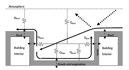 Figure 1. Schematic representation of the urban canyon model. Air circulation is represented by the continuous bold line. Turbulent fluxes are indicated by the resistance network. Thin dashed lines describe conduction through walls, roads and roofs and the bold dashed arrows represent radiative fluxes.
Building shadowing effects are included, together with vegetation (including trees) shadowing effects. Shadowing is represented in terms of sky view factors that depict the area of each urban surface and the sky that is visible by other urban surfaces (e.g., walls and road). Up to 3 reflections of solar radiation from urban surfaces are calculated by the UCM. The sky view factors are modified in the presence of vegetation to reduce the amount of solar radiation reaching the walls. This is achieved by simply raising the canyon floor by the displacement height of the vegetation, thereby obscuring a portion of the wall surface on either side of the canyon.
Latent heat flux for urban areas is calculated as a combination of transpiration from the urban vegetation, evaporation from water on leaves and evaporation from the water on the road and roofs. If the water present on the road or roof is greater than 1 mm, then the excess water is assumed to be removed by drainage. A simple bucket model of soil moisture was found to be adequate for constraining the water availability for transpiration, which balances the budget of rainfall that reaches the surface under the vegetation canopy and the water removed by transpiration.
By modifying the canyon geometries, building material thermal properties and the size of vegetation spaces, tree height etc., the UCM can represent different urban forms, such as a high density CBD, lower density urban fringe, industrial areas or areas of vegetation (e.g., sporting fields and parks). Heat conduction and storage is simulated by separate 3 layers conduction models for roofs, both canyon walls and road surfaces. Different layers have different heat capacity, conductivity and thickness, depending on the building material of that layer (e.g., brick, wood, etc.). The outermost layers are the thinnest, so as to better estimate the skin temperature of the building or road surface. The current study solves for the temperature at each of the 3 layers of the roof, two walls and road surfaces by settingthe interior building temperature to a constant value of 20 °C. Anthropogenic fluxes due to traffic are based on measurements from a Melbourne flux station and vary with the diurnal cycle [48]. Heat is conducted through building walls to couple to the canyon sensible heat flux budget. An idealized model of air conditioning is included to close the urban model energy budget. Excess heat entering the building interior is pumped back into the canyon along with the energy required to pump the heat out of the building as described in Thatcher and Hurley [48]. If an excess of heat is leaving the building interior, then assume an anthropogenic source of heat to warm the building. Although the model also considers the radiative heat transfer inside the canyon between buildings and road surfaces, they are not included in Figure 1 for simplicity.
TAPM is a mesoscale climate model [49] which uses prognostic equations for the conservation of mass, momentum, turbulence, heat and moisture to simulate winds, temperature and specific humidity. It includes physical parameterizations for cloud microphysics (water vapor, cloud water, cloud ice, rain and snow), radiation, and a soil-canopy surface scheme with vegetation overlaying soil for radiation and surface fluxes. TAPM employs a multiple one-way nesting procedure to dynamically downscale synoptic-scale analyses/forecasts which drive the model at the boundaries of the outer grids. Typical nesting steps are 30, 10, 3 and 1 km.
The UCM is coupled to TAPM every simulation physics time step, which is every 300 s for the simulations described in this paper. TAPM and the UCM exchange radiation, sensible heat, latent heat and momentum fluxes, which couples to the TAPM planetary boundary layer turbulence closure parameterization. Details of the UCM and coupling have been reported in Thatcher and Hurley [48]. By coupling the UCM with the TAPM, the coupled UCM-TAPM urban climate model can simulate changes in the local meteorology arising from different urban forms under “observed”synoptic data or under global warming projections. In the UCM-TAPM model, a 1 × 1 km grid tile of the land surface, for example, can be assigned one of 39 surface types that include a wide range of natural and built surface types, e.g., snow, water body, forest, shrub land, grassland, pasture, CBD, urban, industrial, etc. The characteristics of the surface types such as the average building height, building height to street canopy width ratio, tree height, vegetation coverage, leaf area index, surface albedos etc. can be adjusted for specific urban forms. Consequently, the UCM-TAPM urban climate model can be used to explore the effectiveness and resilience of various city planning strategies for present as well as future climates. The UCM-TAPM urban climate model has been validated against the measurements from several urban and rural weather stations and demonstrated good capability in urban scale climate modeling for Australian cities [48].
In this study four horizontally level nesting grids were used in the UCM-TAPM, i.e., 30 x 30 km, 10 x 10 km, 3 x 3 km and 1 x 1 km grids. There are 25 x 25 grids for each horizontal grid level, while the vertical direction has a single grid level with 25 grids which extends to 8 km above the ground. Consequently, the total simulation domain was 750 x 750 x 8 km with a spatial resolution of 1 km around the urban area in interest. Figure 2a illustrates the satellite image of the region approximately 12.5 km from the Melbourne CBD area created by ArcGIS® software by Esri and Figure 2b illustrates this region in the UCM-TAPM 1 x 1 km grid level. It can be seen that the Melbourne CBD area has been approximated by nine 1 x 1 km grids in the UCM-TAPM model.
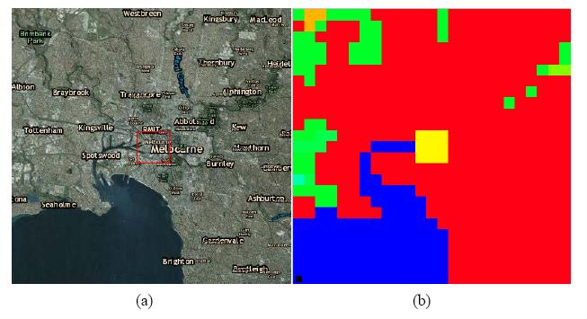 Figure 2. Melbourne CBD representation in the UCM-TAPM: (a) Esri ArcGIS® image; (b) representation in the UCM-TAPM. Here, Yellow: CBD; Blue: Water; Red: generic urban, Green: Shrub land; Brown: Pasture.
In order to investigate the summer cooling potential of vegetation, simulations for the urban climate were carried out using the UCM-TAPM by replacing the Melbourne CBD areas with 10 urban form schemes as shown in Table 1. The CBD form (Urban Form Number 6) in Table 1 represents the existing Melbourne CBD with the vegetation and building coverage percentages estimated from Google images considering that Google images are freely available to the authors. The vegetation and building coverage percentages of the generic urban type in Table 1 (Urban Form Number 5) were based on the measurements for several suburbs in Melbourne as reported by Coutts et al. [52]. Urban Form Number 9, i.e., CBD with 50% green roof, assumes that 50% of the building roofs in the Melbourne CBD area are covered by green roofs. It is noted that to redevelop the Melbourne CBD area into some of the urban form schemes listed in Table 1, such as the forest land (Urban Form Number 1) or grass land (Urban Form Number 3), would be unrealistic in the foreseeable future. However, they are included for better understanding the cooling potential among various urban vegetation schemes in Melbourne CBD.
| a from Coutts et al. [52] b estimated from Google images. Areas other than vegetation and buildings are accounted as roads in the UCM-TAPM c leaf area index for green roof vegetation d estimated average building height divided by the street/road width e rainfall has been modeled and considered in the UCM-TAPM modeling. Irrigation is the additional watering to prevent the vegetation dry out. f GR is the abbreviation for green roof g DV is the abbreviation for double vegetation | ||||||||||
| Urban Form Number | Urban Form | Vegetation Type | Vegetation Area in Entire Land Area (%) | Vegetation Coverage Fraction within Vegetation Area | Leaf Area Index | Green Roof Coverage of Building Roof Area (%) | Estimated Building Coverage Over Entire Land Area (%) | Average Building Height (m) | Estimated Building Height to Canyon Width Ratio d | Irrigation e |
| 1 |
Forest (low sparse) |
low sparse (woodland) | 100 | 0.25 | 2.0 | 0 | 0 | ‒ | ‒ | No |
| 2 | Shrub-land | mid dense (scrub) | 100 | 0.50 | 2.6 | 0 | 0 | ‒ | ‒ | No |
| 3 | Grassland | mid dense tussock | 100 | 0.50 | 1.2 | 0 | 0 | ‒ | ‒ | No |
| 4 | Urban (leafy) | Mixed | 49 | 1.00 | 3 | 0 | 40 | 6.0 | 0.4 | Yes |
| 5 | Urban (generic) | Mixed | 38 a | 1.00 | 3 | 0 | 45 a | 6.0 | 0.4 | Yes |
| 6 | CBD | Mixed | 15 b | 1.00 | 3 | 0 | 65 b | 12.0 | 1.3 | Yes |
| 7 | CBD (with 1/3 Vegetation) | Mixed | 5 | 1.00 | 3 | 0 | 65 | 12.0 | 1.3 | Yes |
| 8 | CBD (double vegetation) | Mixed | 33 | 1.00 | 3 | 0 | 62 | 12.0 | 1.3 | Yes |
| 9 | CBD (50% GR f) | Mixed | 15 | 1.00 | 3, 1.5 c | 50 | 65 | 12.0 | 1.3 | Yes |
| 10 | CBD (DV g + 50% GR f) | Mixed | 33 | 1.00 | 3, 1.5 c | 50 | 62 | 12.0 | 1.3 | Yes |
 DownLoad: CSV
The observed synoptic climate data and global warming projections from General Circulation Model (GCM) were used for simulating the current and future Melbourne climates under various urban forms and vegetation schemes. For the current Melbourne climate simulations, the downscaled climate data from National Centre for Environmental Prediction (NCEP) were used. For future climate projections, the Intergovernmental Panel on Climate Change suggested that due to the varying sets of strengths and weaknesses of various GCMs, no single model can be considered the best. Therefore, multiple GCMs should be used to take into account the uncertainties of the models for impact assessment. In the current study, five GCMs including GFDL2.1, CSIRO-MK3.5, MIROC3.2, ECHAM5 and HadCM3 based on the A2 scenario were used for future Melbourne climate simulations. For each GCM, the future climates at 60 km resolution were obtained using the Conformal Cubic Atmospheric Model (CCAM) [53,54,55,56]. The atmospheric data from the CCAM simulations is then extracted for boundary conditions of the outmost domain for the UCM-TAPM modeling.
Table 2 lists the synoptic climate data sets used in this study with the climate model applied and the year simulated. In total, 11 sets of synoptic climate data were used in this study. The years 2001 and 2009 were chosen to represent current Melbourne climate. The selection of year 2001 in this study was arbitrary. Year 2009 is significant for Melbourne due to the extreme heatwave during the summer 2009. It is noted that single simulation years for individual GCM projections are insufficient to reproduce the climatology of Melbourne in the future. Nevertheless, the yearlong runs are of sufficient length to test the simulated response to changes in urban forms as modeled by UCM-TAPM. Furthermore, as discussed in Section 3, the simulated sensitivity to changes in urban forms was found to be relatively consistent among the different GCM projections and at different levels of global warming. Consequently, multi-year simulations for individual GCM projections, which require substantial more computation resources, were not carried out in the current study.
| Models | Developers | Year simulated |
| Reanalysis data | National Centre for Environmental Prediction (NCEP), USA | 2001, 2009 |
| GFDL2.1 | Geophysical Fluid Dynamics Laboratory (GFDL), USA | 2030, 2047, 2050, 2087, 2090 |
| CSIRO-Mk3.5 | Commonwealth Scientific and Industrial Research Organization, Australia | 2030 |
| MIROC3.2 | Centre for Climate System Research, National Institute for Environmental Studies, and Frontier Research Centre for Global Change, Japan | 2030 |
| ECHAM5 | Max Planck Institute for Meteorology, Germany | 2030 |
| HadCM3 | The Hadley Centre, UK | 2030 |
DownLoad: CSVA total of 110 UCM-TAPM simulations were carried out using the 11 synoptic climate data sets as described in Table 2 and the 10 urban forms as described in Table 1 for the Melbourne CBD area. Each UCM-TAPM simulation took approximately 10 hours using a 2.3 GHz processor. It is noted that like other regional and urban climate models, the UCM-TAPM is aimed for predicting urban climate probability distributions and seasonal variability of the climatic variables [48]. Therefore, it is not intended for predicting short term climate phenomena such as the hourly air temperature or hourly wind speed. In this study, the cooling potential of vegetation on the local climate in the Melbourne CBD area are investigated using the following three summer seasonal air temperatures obtained by the UCM-TAPM simulations:
· TMin: average summer daily minimum temperature (average over January, February and December);
· TMean: average summer mean temperature; and
· TMax: average summer daily maximum temperature;
The cooling potential on TMean for a particular urban form is expressed by the reduction in the average summer mean temperature, i.e., DTMean, which is defined as the reduction in TMean for this particular urban form relative to that for the CBD urban form (Urban Form Number 6 in Table 1) with the same synoptic climate dataset. Similarly, the reduction in the average summer daily minimum and maximum temperatures, i.e., DTMin and DTMax, can be used to quantify the cooling potential of urban vegetation on TMin and TMax, respectively.
Figure 3 shows TMean in 2030, 2047, 2050, 2087 and 2090 for the 10 urban forms obtained using GFDL2.1 projections. Figure 4 shows the TMean results in 2030 projected using different GCMs for the 10 urban forms. In Figures 3 and 4, the TMean results obtained using the NCEP climate datasets for 2001 and 2009 are also included for comparisons. As expected, all the GCMs project an overall warming trend for future summer seasons in the Melbourne CBD in comparison with the current climate represented by 2001 and 2009 in this study. Furthermore, as shown in Figure 4, there are substantial variations in the projected future climates using different GCMs for 2030 for any specific urban form. However, it can be observed that the average summer mean temperature in the Melbourne CBD area reduces with the increase in urban vegetation coverage with the generic urban area predicted to be around 0.5 °C cooler than the existing CBD urban forms. The maximum cooling potential of around 2 °C could be achieved if the CBD area would have been transformed to a natural forest park land. Similar cooling potential for urban vegetation was observed for the corresponding TMean and TMax in the CBD area. These levels of cooling potential appear to be consistent with the range reported by previous researchers [31,32,35,39,40,41,45,46,47].
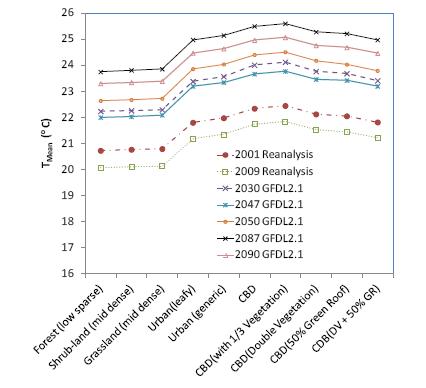 Figure 3. TMean obtained for various urban forms in future climates projected using GFDL2.1.
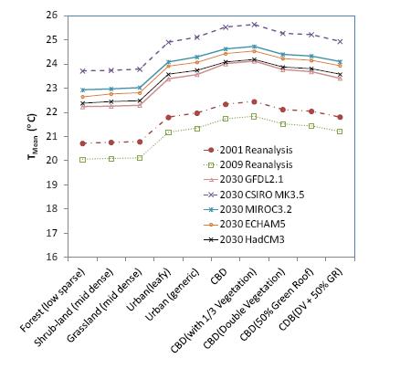 Figure 4. TMean obtained for various urban forms in 2030 projected using different GCMs.
It was also found that the TMean curves in Figures 3 and 4 for different future climates projected by different GCMs are generally parallel to each other. In other words, the cooling potential on the TMean as a result of various urban forms and vegetation schemes does not change significantly with different GCMs and future climate change. This can be better demonstrated with the corresponding DTMin, DTMean and DTMaxresults.
Figures 5a-5c show the DTMin, DTMean and DTMax for various urban forms in 2001 and 2009 using the NECP climate data and in future climates projected using GFDL2.1. Figures 6a-6c show the DTMin, DTMean and DTMax for various urban forms in 2001 and 2009 using the NECP climate data and in 2030 projected using different GCMs. In Figures 5 and 6, the thick solid lines are the mean values of DTMin, DTMean and DTMax for each urban form across the 11 synoptic climatic datasets. It was found that despite the projected warming trends in the future and variations in climate projections using different GCMs, the variations in DTMin, DTMean and DTMax are generally within ± 20% of the means for the 11 synoptic climatic data sets. For a specific urban form, the variation in the DTMean is the smallest, while the variation in DTMin is the largest. It is also seen that the variations in DTMin, DTMean and DTMax generally increase with an increase in the urban vegetation coverage.
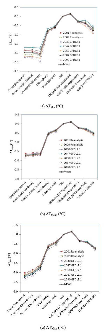 Figure 5. Projections of DTMin, DTMean and DTMax for the 10 urban forms in 2030, 2047, 2050, 2087 and 2090 using GFDL2.1.
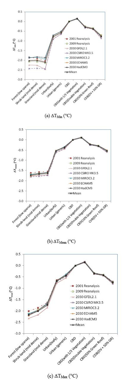 Figure 6. Projections of DTMin, DTMean and DTMax for the 10 urban forms in 2030 using different GCMs.
The cooling potential of urban vegetation is determined by two aspects, vegetation shading and evapotranspiration, with the latter the dominant effect considering that the vegetation shading effect for a specific urban form is more or less fixed. Evapotranspiration rate of urban vegetation scenarios is mainly affected by rainfall. Therefore, it is expected that the variations in the DTMin, DTMean and DTMax are augmentedwith increasing urban vegetation coverage and are highest for the grassland, shrub land and the forest park urban forms (Figures 5 and 6). Compared with the mean values of DTMin, DTMean and DTMax for the 11 synoptic climatic data sets (the thick dotted lines in Figures 5 and 6), the variations in the DTMin, DTMean and DTMax for the grassland, shrub land and the forest park urban forms are within ± 20%, ± 7% and ± 9%, respectively.
The relatively higher variation in DTMin may be explained by the fact that daily minimum temperature occurs during night or early morning when there is no solar radiation which is the major heat source among the urban energy budgets. Cooling through vegetation evapotranspiration, thus, becomes a relatively large heat sink component during night and early morning. Consequently, variations in the rainfall in different years or in the same year projected using different GCMs impact more on TMin than on DTMean and DTMax, although overall, these impacts are limited (Figures 5 and 6).
The relatively insignificant variation in the cooling potential for a specific urban form and vegetation scheme suggests that the cooling potential of urban vegetation in the future can be reasonably envisaged similar to those in the current micro-climate at various urban forms and vegetation schemes. The latter can be obtained with carefully designed experiments by selecting or modifying the urban forms and vegetation schemes in or around an existing city area. For example, temperatures can be monitored simultaneously in existing parks, grassed and planted areas and in highly built-up regions in or near the Melbourne CBD. Such thermal map relationship has been included as one key area of information development for the City of Melbourne’s urban forest strategy [57].
As mentioned in the introduction section, Nicholls et al. [14]reported that, based on historical mortality data, the excess heat related mortality amongst the population over 65 increases rapidly in Melbourne when the daily mean temperatures exceed 30 °C. Therefore, it is useful to examine the cooling benefit of urban vegetation in terms of its impact on the number of hot days with the daily mean temperatures higher than 30°C in a year, defined as DAYSt > 30 °Chereafter.
Figure 7 shows the predicted DAYSt > 30 °C for 2001 and 2009 for various urban forms in the Melbourne CBD. As expected, DAYSt > 30 °Cvaries for different vegetation schemes in different years. The number of the hot days could be reduced up to 82% and 50% with the forest parkland urban form compared to the CBD urban form in 2001 and 2009 respectively. It is also observed that simulated results for 2009 do not show reductions in the DAYSt > 30 °C with several urban vegetation schemes, e.g., the leafy urban form in comparison with the CBD urban form which has a DAYSt > 30 °C at 10:00. Further examination of the simulated temperatures showed that during these 10 hot days, the daily mean temperatures with the leafy urban form are 0.2 to 1.1°C lower than those corresponding days with the CBD urban form. Consequently, although the DAYSt > 30 °C in 2009 may not be affected by urban vegetation, the severity of the urban heat stress is predicted to be reduced by urban vegetation during these hot days.
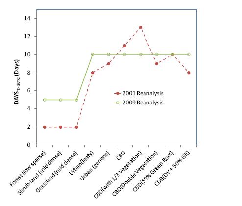 Figure 7. Projected number of days with the daily mean temperatures higher than 30 °C in 2001 and 2009.
Figure 8 shows the DAYSt > 30 °Cresults for 2030, 2047, 2087 and 2090 projected by GFDL2.1 with various urban vegetation schemes. Dependent on the specific year simulated, the number of hot days can vary significantly, although urban vegetation generally projected to reduce the DAYSt > 30 °C in Melbourne (Figure 8). For a warm year with high number of DAYSt > 30 °C, e.g., in 2087, the reduction in the DAYSt > 30 °C is projected to be 26% and 66% for the leafy urban and forest parkland, respectively, when compared to the CBD urban form. In average, the leafy urban vegetation scheme is projected to reduce around 20% hot days when compared with the CBD urban form.
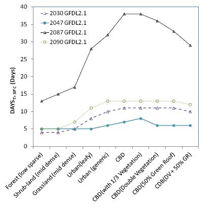 Figure 8. Projected number of days with the daily mean temperatures higher than 30 °C for different years using GFDL2.1.
It should be emphasized that the results obtained using urban climate models should be considered as long term averages and statistical trends only. Consequently, the DAYSt > 30 °C values presented should not be taken as the exact number of days with daily mean temperature above 30 °C for a specific year simulated. It should be interpreted as a potential long term trend projected by a specific GCM in the Melbourne CBD.
It is also understood that healthy urban vegetation requires adequate available water resources and irrigations. Consequently, an indispensable part of the City of Melbourne’s urban forest strategy is developing water sensitive urban designs by better managing stormwater with wetlands, underground tanks and increasing permeable surfaces etc. [57].
Summer cooling potential of various urban forms and vegetation schemes were investigated using an urban climate model for the current and future climates, also using multiple GCMs by replacing the Melbourne CBD area with 10 urban forms. It was found that the average seasonal summer temperatures such as the average summer daily minimum, mean and maximum temperatures can be reduced in the range of around 0.5 to 2 °C by replacing the Melbourne CBD with more vegetated suburbs and planted parklands, respectively. Increasing in urban vegetation is predicted to lead to the reduction in the number of hot days or the severity of these hot days.
It was also found that despite projected climate warming in the future and significant variations in the climate projections among different GCMs, the cooling potential in terms of the reduction in the average summer daily minimum, mean and maximum temperatures due to various urban forms and vegetation schemes remains reasonably unchanged in comparison with those predicted for the present climate. This finding may have the following implications or applications:
1) In terms of the average seasonal summer temperatures, the cooling potential of urban vegetation in the current climate may be obtained with carefully designed experiments by selecting or modifying the urban forms and vegetation schemes in or around an existing city area. The cooling potential of urban vegetation in the future can be reasonably envisaged similar to those in the current climate at various urban forms and vegetation schemes.
2) When using urban climate modeling for investigating the summer cooling potential in terms of DTMin, DTMean and DTMax with various urban forms and urban vegetation schemes, the choice of GCMs or the selection of specific current or future year is less important. In other words, the summer cooling potential of a specific urban form can be reasonably estimated by running simulations for several selected years with one or a few GCMs.
3) Although urban vegetation leads to the reduction in hot days with daily mean temperature above 30 °C in the Melbourne CBD, the benefit of urban vegetation can be significantly different among different years. Nevertheless, urban vegetation is projected to reduce the severity of urban heat stress during future hot days in the Melbourne CBD. On average, the leafy urban vegetation scheme is projected to reduce hot days by around 20% when compared with the CBD urban form.
This study was partly funded by the Horticulture Australia Limited using the Nursery Industry Levy (Project # NY 11013 and NY12018) and CSIRO Climate Adaptation Flagship.
All authors declare no conflicts of interest in this paper.
| [1] | United Nations, World Urbanization Prospects, the 2014 Revision. 2014. Available from: http://esa.un.org/unpd/ accessed March 2015. |
| [2] | DSEWPaC (Department of Sustainability, Environment, Water, Population and Communities), State of the Environment 2011, 2011. Available from: http://www.environment.gov.au/science/soe/2011-report/contents |
| [3] |
Morris CJG, Simmonds I, Plummer N (2001) Quantification of the Influences of Wind and Cloud on the Nocturnal Urban Heat Island of a Large City. J Appl Meteorol 40: 169-182. doi: 10.1175/1520-0450(2001)040<0169:QOTIOW>2.0.CO;2

|
| [4] |
Coutts A, Beringer J, Tapper N (2010) Changing urban climate and CO2 emissions: implications for the development of policies for sustainable cities. Urban Policy Res 28: 27-47. doi: 10.1080/08111140903437716
|
| [5] |
Wu K, Yang XQ (2013) Urbanization and heterogeneous surface warming in eastern China. Chin Sci Bull 58: 1363-1373. doi: 10.1007/s11434-012-5627-8
|
| [6] | DSE (Department of Sustainability and Environment), Melbourne 2030: Planning for Sustainable Growth. State Government of Victoria, 2002. Available from: http://www.dtpli.vic.gov.au/planning/plans-and-policies/planning-for-melbourne/melbournes-strategic-planning-history/melbourne-2030-planning-for-sustainable-growth |
| [7] | Konopacki S, Akbari H (2002) Energy savings for heat island reduction strategies in Chicago and Houston (including updates for Baton Rouge, Sacramento, and Salt Lake City). Draft Final Report, LBNL-49638, University of California, Berkeley. |
| [8] |
Kolokotroni M, Giannitsaris I, Watkins R (2006) The effect of the London Urban Heat Island on building summer cooling demand and night ventilation strategies. Sol Energ 80: 383-392. doi: 10.1016/j.solener.2005.03.010
|
| [9] | Priyadarsini R (2011) Urban Heat Island and its Impact on Building Energy Consumption. Adv Build Energ Res 3: 261-270. |
| [10] |
Changnon SA, Kunkel KE, Reinke BC (1996) Impacts and responses to the 1995 heat wave: A call to action. Bull Am Meteorol Soc 77: 1497-1505. doi: 10.1175/1520-0477(1996)077<1497:IARTTH>2.0.CO;2
|
| [11] |
Haines A, Kovats RS, Campbell-Lendrum D, et al. (2006) Climate change and human health: impacts, vulnerability, and mitigation. Lancet 367: 2101-2109. doi: 10.1016/S0140-6736(06)68933-2
|
| [12] |
Cadot E, Rodwin VG, Spira A (2007) In the heat of the summer: lessons from the heat waves in Paris. J Urban Health 84: 466-468. doi: 10.1007/s11524-007-9161-y
|
| [13] | Luber G (2008) Climate Change and Extreme Heat Events, Am J Prev Med 35: 429-435. |
| [14] | Nicholls N, Skinner C, Loughnan M, et al. (2008) A simple heat alert system for Melbourne, Australia, Int J Biometeorol 52: 375-384. |
| [15] |
Kovats RS, Hajat S (2008) Heat stress and public health: a critical review. Annu Rev Public Health 29: 41-55. doi: 10.1146/annurev.publhealth.29.020907.090843
|
| [16] |
Loughnan ME, Nicholls N, Tapper NJ (2010) The effects of summer temperature, age and socioeconomic circumstance on acute myocardial infarction admissions in Melbourne, Australia. Int J Health Geogr 9: 41. doi: 10.1186/1476-072X-9-41
|
| [17] | DHS, January 2009 Heatwave in Victoria: an assessment of health impacts. Victorian Government Department of Human Services, Victoria, 2009. Available from: http://docs.health.vic.gov.au/docs/doc/F7EEA4050981101ACA257AD80074AE8B/$FILE/heat_health_impact_rpt_Vic2009.pdf |
| [18] | Alexander LV, Arblaster J (2008) Assessing trends in observed and modelled climate extremes over Australia in relation to future projections. Int J Climatol 29: 417-435. |
| [19] | Solecki WD, Rosenzweig C, Parshall L, et al. (2005) Mitigation of the heat island effect in urban New Jersey. Global Environ Chang Part B: Environ Hazards 6: 39-49. |
| [20] |
Gill SE, Handley JF, Ennos AR, et al. (2008) Characterising the urban environment of UK cities and towns: A template for landscape planning. Landscape Urban Plann 87: 210-222. doi: 10.1016/j.landurbplan.2008.06.008
|
| [21] |
Gaitani N, Spanou A, Saliari M, et al. (2011) Improving the microclimate in urban areas: a case study in the centre of Athens. Build Serv Eng Res Technol 32: 53-71. doi: 10.1177/0143624410394518
|
| [22] |
Kleerekoper L, van Esch M, Salcedo TB (2012) How to make a city climate proof, addressing the urban heat island effect. Resour Conserv Recycl 64: 30-38. doi: 10.1016/j.resconrec.2011.06.004
|
| [23] | DCLG, Building a greener future: towards zero carbon development. UK: Department of Communities and Local Government, 2007. Available from: http://webarchive.nationalarchives.gov.uk/20120919132719/http://www.communities.gov.uk/documents/planningandbuilding/pdf/153125.pdf |
| [24] | European Commission, Low energy buildings in Europe: current state of play, definition and best practice. 2009. Available from:http: //regions202020.eu/cms/inspiration/resources/PublicResource/330/view |
| [25] |
Wang XM, Chen D, Ren ZG (2010) Assessment of climate change impact on residential building heating and cooling energy requirement in Australia. Build Environ 45: 1663-1682. doi: 10.1016/j.buildenv.2010.01.022
|
| [26] |
Rosenfeld AH, Akbari H, Romm JJ, et al. (1998) Cool communities: strategies for heat island mitigation and smog reduction. Energ Build 28: 51-62. doi: 10.1016/S0378-7788(97)00063-7
|
| [27] |
Akbari H, Pomerantz M, Taha H (2001) Cool surfaces and shade trees to reduce energy use and improve air quality in urban areas. Sol Energ 70: 295-310. doi: 10.1016/S0038-092X(00)00089-X
|
| [28] | U.S. Environmental Protection Agency, Reducing Urban Heat Islands: Compendium of Strategies. 2008. Available from: http: //www.epa.gov/hiri/resources/compendium.htm |
| [29] |
Memon RA, Leung DYC, Liu CH (2008) A review on the generation, determination and mitigation of Urban Heat Island. J Environ Sci 20: 120-128. doi: 10.1016/S1001-0742(08)60019-4
|
| [30] | Santamouris M (2012) Cooling the cities - a review of reflective and green roof mitigation technologies to fight heat island and improve comfort in urban environments. Sol Energ 103: 680-703. |
| [31] | Liu K, Bass B (2005) Performance of Green Roof Systems. National Research Council Canada, Report No. NRCC-47705, Toronto, Canada. |
| [32] | Rosenzweig C, Solecki W, Parshall L, et al. (2006) Mitigating New York City's Heat Island with Urban Forestry, Living Roofs, and Light Surfaces. Sixth Symposium on the Urban Environment and Forum on Managing our Physical and Natural Resources, American Meteorological Society, Atlanta, GA. |
| [33] |
Alexandri E, Jones P (2008) Temperature decreases in an urban canyon due to green walls and green roofs in diverse climates. Build Environ 43: 480-493. doi: 10.1016/j.buildenv.2006.10.055
|
| [34] | Wong JKW, Lau LSK (2013) From the ‘urban heat island’ to the ‘green island’? A preliminary investigation into the potential of retrofitting green roofs in Mongkok district of Hong Kong. Habit Int 39: 25-35. |
| [35] | Susca T, Gaffin SR, Dell'Osso GR (2011) Positive effects of vegetation: Urban heat island and green roofs, Environ Pollut 159: 2119-2126. |
| [36] | Xu T, Sathaye J, Akbari H, et al. (2012) Quantifying the direct benefits of cool roofs in an urban setting: Reduced cooling energy use and lowered greenhouse gas emissions. Build Environ 48: 1-6. |
| [37] |
Smith GB, Aguilar JLC, Gentle AR, et al. (2012) Multi-parameter sensitivity analysis: A design methodology applied to energy efficiency in temperate climate houses. Energy Build 55: 668-673. doi: 10.1016/j.enbuild.2012.09.007
|
| [38] | Bozonnet E, Musy M, Calmet I, et al. (2013) Modeling methods to assess urban fluxes and heat island mitigation measures from street to city scale. Int J Low Carbon Technol 0: 1-16. |
| [39] |
Sailor DJ (1995) Simulated urban response to modifications in surface albedo and vegetative cover. J Appl Meteor 34: 1694- 1704. doi: 10.1175/1520-0450-34.7.1694
|
| [40] |
Taha H, Douglas S, Haney J (1997) Mesoscale meteorological and air quality impacts of increased urban albedo and vegetation. Energ Build 25: 169-177. doi: 10.1016/S0378-7788(96)01006-7
|
| [41] |
Shashua-Bar L, Hoffman ME (2000) Vegetation as a climatic component in the design of an urban street: An empirical model for predicting the cooling effect of urban green areas with trees. Energy Build 31: 221-35. doi: 10.1016/S0378-7788(99)00018-3
|
| [42] |
Kong FH, Yin HW, Wang CZ, et al. (2014) A satellite image-based analysis of factors contributing to the green-space cool island intensity on a city scale. Urban For Urban Gree 13: 846-853. doi: 10.1016/j.ufug.2014.09.009
|
| [43] |
Perini K, Magliocco A (2014) Effects of vegetation, urban density, building height, and atmospheric conditions on local temperatures and thermal comfort. Urban For Urban Gree 13:495-506. doi: 10.1016/j.ufug.2014.03.003
|
| [44] |
Chen C, Yue Y, Jiang W (2014) Numerical Simulation on Cooling Effects of Greening for Alleviating Urban Heat Island Effect in North China. Appl Mech Mater 675-677: 1227-1233. doi: 10.4028/www.scientific.net/AMM.675-677.1227
|
| [45] |
Yang JB, Liu HN, Sun JN, et al. (2015) Further Development of the Regional Boundary Layer Model to Study the Impacts of Greenery on the Urban Thermal Environment. J Appl Meteor Climatol 54: 137-152. doi: 10.1175/JAMC-D-14-0057.1
|
| [46] | Gromke C, Blocken B, Janssen W, et al. (2015) CFD analysis of transpirational cooling by vegetation: Case study for specific meteorological conditions during a heat wave in Arnhem, Netherlands, Build Environ 83: 11-26. |
| [47] |
Middel A, Chhetri N, Quay R (2015) Urban forestry and cool roofs: Assessment of heat mitigation strategies in Phoenix residential neighborhoods. Urban For Urban Gree 14: 178-186. doi: 10.1016/j.ufug.2014.09.010
|
| [48] |
Thatcher M, Hurley P (2012) Simulating Australian urban climate in a mesoscale atmospheric numerical model. Boundary Layer Meteorol 142: 149-175. doi: 10.1007/s10546-011-9663-8
|
| [49] |
Hurley P, Physick W, Luhar A (2005) TAPM - A practical approach to prognostic meteorological and air pollution modeling. Environ Model Sotfw 20: 737-752. doi: 10.1016/j.envsoft.2004.04.006
|
| [50] |
Masson V (2000) A physically-based scheme for the urban energy budget in atmospheric models. Boundary Layer Meteorol 94: 357-397. doi: 10.1023/A:1002463829265
|
| [51] |
Harman I, Barlow J, Belcher S (2004) Scalar fluxes from urban street canyons. Part II: Model. Boundary Layer Meteorol 113: 387-409. doi: 10.1007/s10546-004-6205-7
|
| [52] |
Coutts A, Beringer J, Tapper N (2007) Impact of increasing urban density on local climate: spatial and temporal variations in the surface energy balance in Melbourne, Australia. J Appl Meteor Climatol 46: 477-493. doi: 10.1175/JAM2462.1
|
| [53] | McGregor J, C-CAM: Geometric aspects and dynamical formulation. CSIRO Atmospheric Research, 2005. Available from: www.cmar.csiro.au/e-print/open/mcgregor_2005a.pdf |
| [54] | McGregor J, Dix M (2008) An updated description of the conformal-cubic atmospheric model. High Resolution Simulation of the Atmosphere and Ocean, Hamilton, K. and Ohfuchi, W., Eds., Springer 51-76. |
| [55] | Katzfey J, McGregor J, Nguyen K, et al. Dynamical downscaling techniques: impacts on regional climate change signals. In: Anderssen RS, Braddock RD and Newham LTH (ed) 18th World IMACS congress and MODSIM09 international congress on modelling and simulation. 2009, July; Cairns. Modelling and Simulation Society of Australia and New Zealand. pp 2377-2383. |
| [56] | Nguyen K, Katzfey J, McGregor J (2011) Global 60 km simulations with the Conformal Cubic Atmospheric Model: Evaluation over the tropics. Clim Dyn 39: 637-654. |
| [57] | City of Melbourne, Urban Forest Strategy Make a Great City Greener 2013-2032. 2015. Available from: http://www.melbourne.vic.gov.au/Sustainability/UrbanForest/Documents/Urban_Forest_Strategy.pdf |
| 1. | Alessio Russo, Giuseppe T. Cirella, 2020, Chapter 10, 978-981-15-3048-7, 187, 10.1007/978-981-15-3049-4_10 | |
| 2. | Sarah Chapman, Marcus Thatcher, Alvaro Salazar, James E.M. Watson, Clive A. McAlpine, The impact of climate change and urban growth on urban climate and heat stress in a subtropical city, 2019, 39, 0899-8418, 3013, 10.1002/joc.5998 | |
| 3. | Mary Thornbush, Urban greening for low carbon cities—introduction to the special issue, 2016, 3, 2372-0352, 133, 10.3934/environsci.2016.1.133 | |
| 4. | Sarah Chapman, Marcus Thatcher, Alvaro Salazar, James E. M. Watson, Clive A. McAlpine, The Effect of Urban Density and Vegetation Cover on the Heat Island of a Subtropical City, 2018, 57, 1558-8424, 2531, 10.1175/JAMC-D-17-0316.1 | |
| 5. | Komali Yenneti, Lan Ding, Deo Prasad, Giulia Ulpiani, Riccardo Paolini, Shamila Haddad, Mattheos Santamouris, Urban Overheating and Cooling Potential in Australia: An Evidence-Based Review, 2020, 8, 2225-1154, 126, 10.3390/cli8110126 | |
| 6. | Prabhasri Herath, Marcus Thatcher, Huidong Jin, Xuemei Bai, Effectiveness of urban surface characteristics as mitigation strategies for the excessive summer heat in cities, 2021, 72, 22106707, 103072, 10.1016/j.scs.2021.103072 | |
| 7. | Mary J. Thornbush, Introducing the Special Issue on Urban Sustainability Futures, 2022, 14, 2071-1050, 11964, 10.3390/su141911964 |


Figures(8) / Tables(2)

Dong Chen, Marcus Thatcher, Xiaoming Wang, Guy Barnett, Anthony Kachenko, Robert Prince. Summer cooling potential of urban vegetation—a modeling study for Melbourne, Australia[J]. AIMS Environmental Science, 2015, 2(3): 648-667. doi: 10.3934/environsci.2015.3.648

| a from Coutts et al. [52] b estimated from Google images. Areas other than vegetation and buildings are accounted as roads in the UCM-TAPM c leaf area index for green roof vegetation d estimated average building height divided by the street/road width e rainfall has been modeled and considered in the UCM-TAPM modeling. Irrigation is the additional watering to prevent the vegetation dry out. f GR is the abbreviation for green roof g DV is the abbreviation for double vegetation | ||||||||||
| Urban Form Number | Urban Form | Vegetation Type | Vegetation Area in Entire Land Area (%) | Vegetation Coverage Fraction within Vegetation Area | Leaf Area Index | Green Roof Coverage of Building Roof Area (%) | Estimated Building Coverage Over Entire Land Area (%) | Average Building Height (m) | Estimated Building Height to Canyon Width Ratio d | Irrigation e |
| 1 |
Forest (low sparse) |
low sparse (woodland) | 100 | 0.25 | 2.0 | 0 | 0 | ‒ | ‒ | No |
| 2 | Shrub-land | mid dense (scrub) | 100 | 0.50 | 2.6 | 0 | 0 | ‒ | ‒ | No |
| 3 | Grassland | mid dense tussock | 100 | 0.50 | 1.2 | 0 | 0 | ‒ | ‒ | No |
| 4 | Urban (leafy) | Mixed | 49 | 1.00 | 3 | 0 | 40 | 6.0 | 0.4 | Yes |
| 5 | Urban (generic) | Mixed | 38 a | 1.00 | 3 | 0 | 45 a | 6.0 | 0.4 | Yes |
| 6 | CBD | Mixed | 15 b | 1.00 | 3 | 0 | 65 b | 12.0 | 1.3 | Yes |
| 7 | CBD (with 1/3 Vegetation) | Mixed | 5 | 1.00 | 3 | 0 | 65 | 12.0 | 1.3 | Yes |
| 8 | CBD (double vegetation) | Mixed | 33 | 1.00 | 3 | 0 | 62 | 12.0 | 1.3 | Yes |
| 9 | CBD (50% GR f) | Mixed | 15 | 1.00 | 3, 1.5 c | 50 | 65 | 12.0 | 1.3 | Yes |
| 10 | CBD (DV g + 50% GR f) | Mixed | 33 | 1.00 | 3, 1.5 c | 50 | 62 | 12.0 | 1.3 | Yes |
DownLoad: CSV| Models | Developers | Year simulated |
| Reanalysis data | National Centre for Environmental Prediction (NCEP), USA | 2001, 2009 |
| GFDL2.1 | Geophysical Fluid Dynamics Laboratory (GFDL), USA | 2030, 2047, 2050, 2087, 2090 |
| CSIRO-Mk3.5 | Commonwealth Scientific and Industrial Research Organization, Australia | 2030 |
| MIROC3.2 | Centre for Climate System Research, National Institute for Environmental Studies, and Frontier Research Centre for Global Change, Japan | 2030 |
| ECHAM5 | Max Planck Institute for Meteorology, Germany | 2030 |
| HadCM3 | The Hadley Centre, UK | 2030 |
DownLoad: CSV| a from Coutts et al. [52] b estimated from Google images. Areas other than vegetation and buildings are accounted as roads in the UCM-TAPM c leaf area index for green roof vegetation d estimated average building height divided by the street/road width e rainfall has been modeled and considered in the UCM-TAPM modeling. Irrigation is the additional watering to prevent the vegetation dry out. f GR is the abbreviation for green roof g DV is the abbreviation for double vegetation | ||||||||||
| Urban Form Number | Urban Form | Vegetation Type | Vegetation Area in Entire Land Area (%) | Vegetation Coverage Fraction within Vegetation Area | Leaf Area Index | Green Roof Coverage of Building Roof Area (%) | Estimated Building Coverage Over Entire Land Area (%) | Average Building Height (m) | Estimated Building Height to Canyon Width Ratio d | Irrigation e |
| 1 |
Forest (low sparse) |
low sparse (woodland) | 100 | 0.25 | 2.0 | 0 | 0 | ‒ | ‒ | No |
| 2 | Shrub-land | mid dense (scrub) | 100 | 0.50 | 2.6 | 0 | 0 | ‒ | ‒ | No |
| 3 | Grassland | mid dense tussock | 100 | 0.50 | 1.2 | 0 | 0 | ‒ | ‒ | No |
| 4 | Urban (leafy) | Mixed | 49 | 1.00 | 3 | 0 | 40 | 6.0 | 0.4 | Yes |
| 5 | Urban (generic) | Mixed | 38 a | 1.00 | 3 | 0 | 45 a | 6.0 | 0.4 | Yes |
| 6 | CBD | Mixed | 15 b | 1.00 | 3 | 0 | 65 b | 12.0 | 1.3 | Yes |
| 7 | CBD (with 1/3 Vegetation) | Mixed | 5 | 1.00 | 3 | 0 | 65 | 12.0 | 1.3 | Yes |
| 8 | CBD (double vegetation) | Mixed | 33 | 1.00 | 3 | 0 | 62 | 12.0 | 1.3 | Yes |
| 9 | CBD (50% GR f) | Mixed | 15 | 1.00 | 3, 1.5 c | 50 | 65 | 12.0 | 1.3 | Yes |
| 10 | CBD (DV g + 50% GR f) | Mixed | 33 | 1.00 | 3, 1.5 c | 50 | 62 | 12.0 | 1.3 | Yes |
| Models | Developers | Year simulated |
| Reanalysis data | National Centre for Environmental Prediction (NCEP), USA | 2001, 2009 |
| GFDL2.1 | Geophysical Fluid Dynamics Laboratory (GFDL), USA | 2030, 2047, 2050, 2087, 2090 |
| CSIRO-Mk3.5 | Commonwealth Scientific and Industrial Research Organization, Australia | 2030 |
| MIROC3.2 | Centre for Climate System Research, National Institute for Environmental Studies, and Frontier Research Centre for Global Change, Japan | 2030 |
| ECHAM5 | Max Planck Institute for Meteorology, Germany | 2030 |
| HadCM3 | The Hadley Centre, UK | 2030 |


