The impact of different compression ratios on emissions, and combustion characteristics of a biodiesel engine

Hussein A. Mahmood; Ali O. Al-Sulttani; Hayder A. Alrazen; Osam H. Attia; Hussein A. Mahmood; Ali O. Al-Sulttani; Hayder A. Alrazen; Osam H. Attia

doi:10.3934/energy.2024043

AIMS Energy

2024, Volume 12, Issue 5: 924-945. doi: 10.3934/energy.2024043

Previous Article Next Article

Research article

The impact of different compression ratios on emissions, and combustion characteristics of a biodiesel engine

1.
Department of Reconstruction and Projects, University of Baghdad, Baghdad, Iraq
2.
Department of Water Resources Engineering, College of Engineering, University of Baghdad, Baghdad, Iraq
3.
School of Mechanical and Mining Engineering, University of Queensland, QLD, 4072, Australia

Received: 29 March 2024 Revised: 15 July 2024 Accepted: 05 August 2024 Published: 12 August 2024

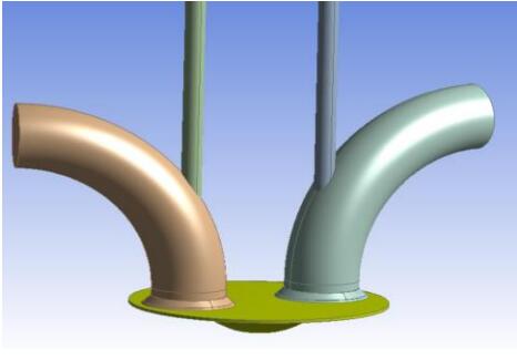
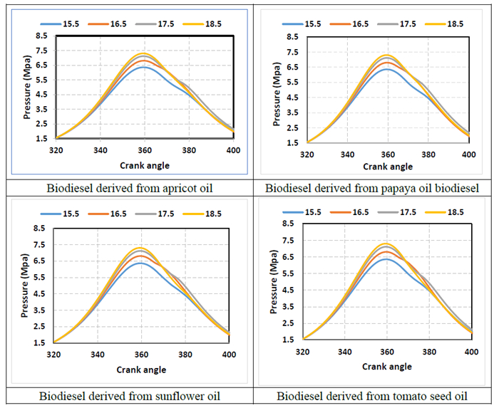
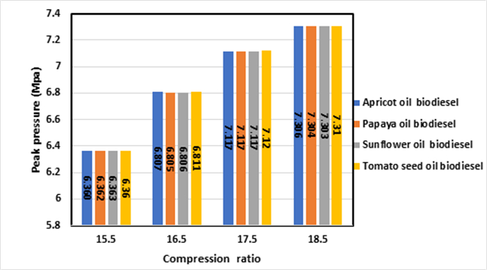
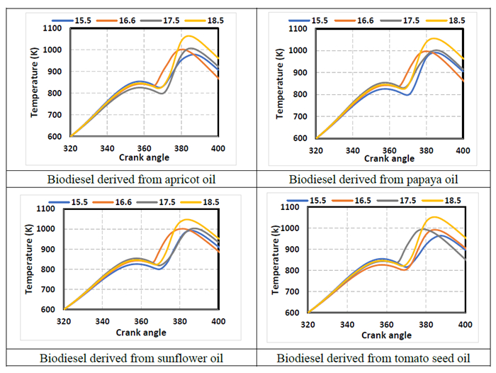
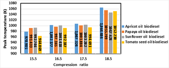
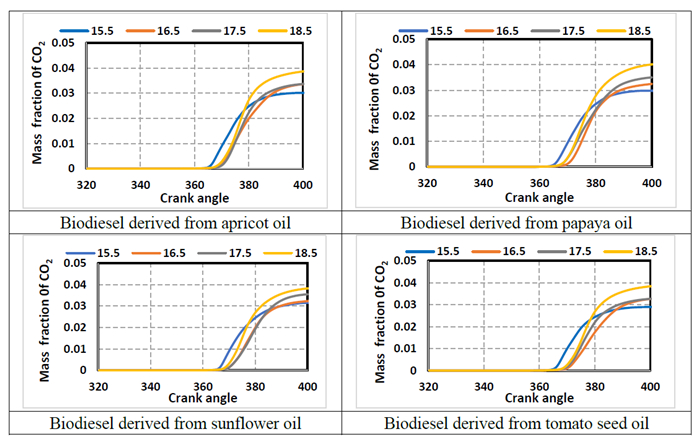
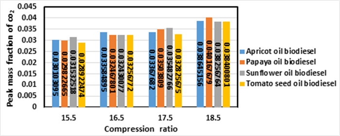
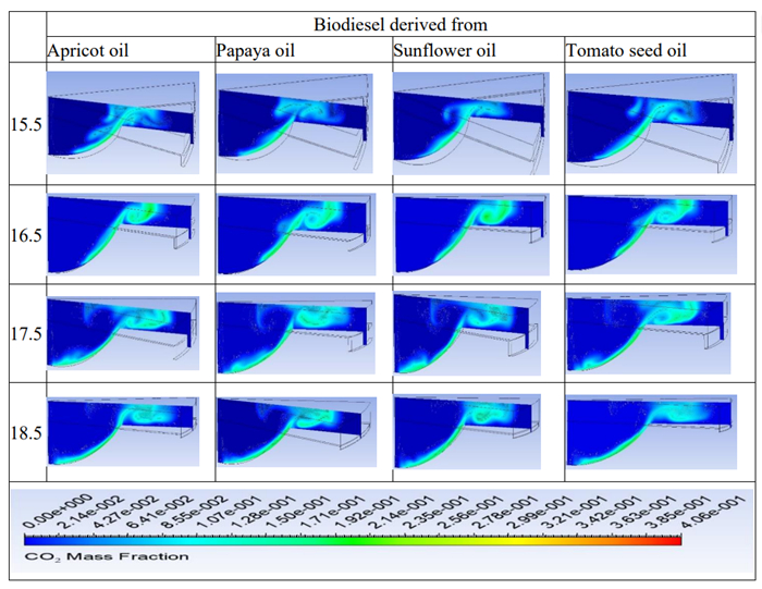
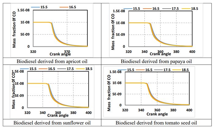
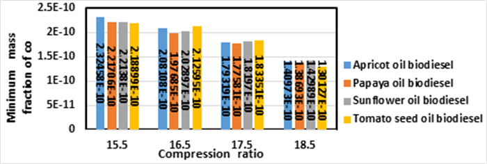
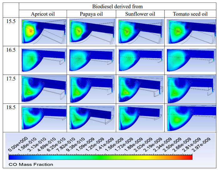
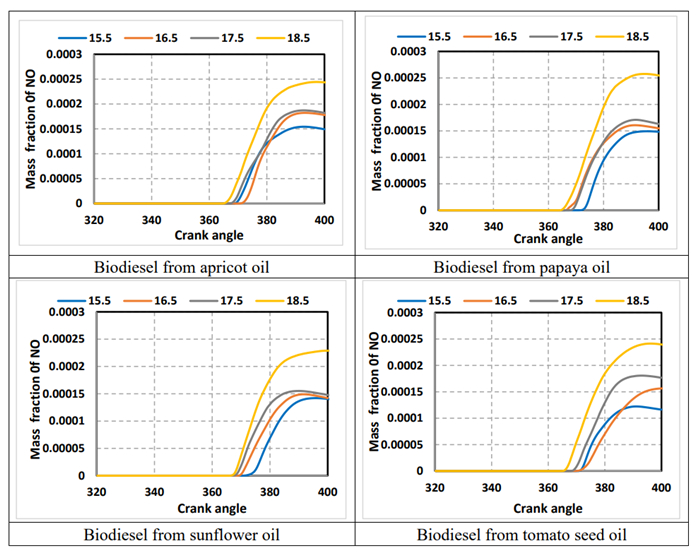
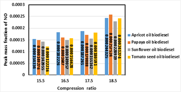
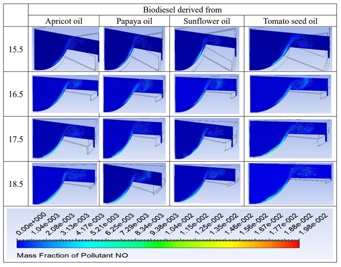
The current work investigated the combustion efficiency of biodiesel engines under diverse ratios of compression (15.5, 16.5, 17.5, and 18.5) and different biodiesel fuels produced from apricot oil, papaya oil, sunflower oil, and tomato seed oil. The combustion process of the biodiesel fuel inside the engine was simulated utilizing ANSYS Fluent v16 (CFD). On AV1 diesel engines (Kirloskar), numerical simulations were conducted at 1500 rpm. The outcomes of the simulation demonstrated that increasing the compression ratio (CR) led to increased peak temperature and pressures in the combustion chamber, as well as elevated levels of CO₂ and NO mass fractions and decreased CO emission values under the same biodiesel fuel type. Additionally, the findings revealed that the highest cylinder temperature was 1007.32 K and the highest cylinder pressure was 7.3 MPa, achieved by biodiesel derived from apricot oil at an 18.5% compression ratio. Meanwhile, the highest NO and CO₂ mass fraction values were 0.000257524 and 0.040167679, respectively, obtained from biodiesel derived from papaya oil at an 18.5% compression ratio. This study explained that the apricot oil biodiesel engine had the highest combustion efficiency with high emissions at a compression ratio of 18:5. On the other hand, tomato seed oil biodiesel engines had low combustion performance and low emissions of NO and CO₂ at a compression ratio of 15:5. The current study concluded that apricot oil biodiesel may be a suitable alternative to diesel fuel operated at a CR of 18:1.

Keywords:

Citation: Hussein A. Mahmood, Ali O. Al-Sulttani, Hayder A. Alrazen, Osam H. Attia. The impact of different compression ratios on emissions, and combustion characteristics of a biodiesel engine[J]. AIMS Energy, 2024, 12(5): 924-945. doi: 10.3934/energy.2024043

Related Papers:

[1]	Qun Dai, Shidong Liu . Stability of the mixed Caputo fractional integro-differential equation by means of weighted space method. AIMS Mathematics, 2022, 7(2): 2498-2511. doi: 10.3934/math.2022140
[2]	Thabet Abdeljawad, Sabri T. M. Thabet, Imed Kedim, Miguel Vivas-Cortez . On a new structure of multi-term Hilfer fractional impulsive neutral Levin-Nohel integrodifferential system with variable time delay. AIMS Mathematics, 2024, 9(3): 7372-7395. doi: 10.3934/math.2024357
[3]	Choukri Derbazi, Zidane Baitiche, Mohammed S. Abdo, Thabet Abdeljawad . Qualitative analysis of fractional relaxation equation and coupled system with Ψ-Caputo fractional derivative in Banach spaces. AIMS Mathematics, 2021, 6(3): 2486-2509. doi: 10.3934/math.2021151
[4]	J. Vanterler da C. Sousa, E. Capelas de Oliveira, F. G. Rodrigues . Ulam-Hyers stabilities of fractional functional differential equations. AIMS Mathematics, 2020, 5(2): 1346-1358. doi: 10.3934/math.2020092
[5]	Kaihong Zhao, Shuang Ma . Ulam-Hyers-Rassias stability for a class of nonlinear implicit Hadamard fractional integral boundary value problem with impulses. AIMS Mathematics, 2022, 7(2): 3169-3185. doi: 10.3934/math.2022175
[6]	Jiqiang Zhang, Siraj Ul Haq, Akbar Zada, Ioan-Lucian Popa . Stieltjes integral boundary value problem involving a nonlinear multi-term Caputo-type sequential fractional integro-differential equation. AIMS Mathematics, 2023, 8(12): 28413-28434. doi: 10.3934/math.20231454
[7]	Hasanen A. Hammad, Hassen Aydi, Hüseyin Işık, Manuel De la Sen . Existence and stability results for a coupled system of impulsive fractional differential equations with Hadamard fractional derivatives. AIMS Mathematics, 2023, 8(3): 6913-6941. doi: 10.3934/math.2023350
[8]	Dongming Nie, Usman Riaz, Sumbel Begum, Akbar Zada . A coupled system of $p$ -Laplacian implicit fractional differential equations depending on boundary conditions of integral type. AIMS Mathematics, 2023, 8(7): 16417-16445. doi: 10.3934/math.2023839
[9]	Thanin Sitthiwirattham, Rozi Gul, Kamal Shah, Ibrahim Mahariq, Jarunee Soontharanon, Khursheed J. Ansari . Study of implicit-impulsive differential equations involving Caputo-Fabrizio fractional derivative. AIMS Mathematics, 2022, 7(3): 4017-4037. doi: 10.3934/math.2022222
[10]	Subramanian Muthaiah, Dumitru Baleanu, Nandha Gopal Thangaraj . Existence and Hyers-Ulam type stability results for nonlinear coupled system of Caputo-Hadamard type fractional differential equations. AIMS Mathematics, 2021, 6(1): 168-194. doi: 10.3934/math.2021012

Abstract

1. Introduction

Fractional differential equations have played an important role and have presented valuable tools in the modeling of many phenomena in various fields of science and engineering ^{[6,7,8,9,10,11,12,13,14,15,16]}. There has been a significant development in fractional differential equations in recent decades ^{[2,3,4,5,26,23,33,37]}. On the other hand, many authors studied the stability of functional equations and established some types of Ulam stability ^{[1,17,18,19,20,21,22,24,27,28,29,30,31,32,33,34,35,36,37]} and references there in. Moreover, many authors discussed local and global attractivity ^{[8,9,10,11,34]}.

Benchohra et al. ^[13] established some types of Ulam-Hyers stability for an implicit fractional-order differential equation.

A. Baliki et al. ^[11] have given sufficient conditions for existence and attractivity of mild solutions for second order semi-linear functional evolution equation in Banach spaces using Schauder's fixed point theorem.

Benchohra et al. ^[15] studied the existence of mild solutions for a class of impulsive semilinear fractional differential equations with infinite delay and non-instantaneous impulses in Banach spaces. This results are obtained using the technique of measures of noncompactness.

Motivated by these works, in this paper, we investigate the following initial value problem for an implicit fractional-order differential equation

$\begin{align} \left\{ \begin{array}{c} ^C\mathfrak{D}^\alpha \left[ \mathfrak{x}(\mathfrak{t})- \mathfrak{h}(\mathfrak{t}, \mathfrak{x}(\mathfrak{t}))\right] = \mathfrak{g}_1( \mathfrak{t}, \mathfrak{x}(\mathfrak{t}), \mathfrak{I}^\mathfrak{\beta} \mathfrak{g}_2(\mathfrak{t}, \mathfrak{x}(\mathfrak{t}))) \; \; \; \mathfrak{t}\in {J}, \; 1 \lt \alpha \leq 2 , \; \alpha \geq \beta, \\\\ \bigg(\mathfrak{x}(\mathfrak{t})- \mathfrak{h}(\mathfrak{t}, \mathfrak{x}(t))\bigg)\bigg|_{\mathfrak{t} = 0} = 0\; \; \; \; \mbox{and}\; \; \; \; \; \frac{d}{d\mathfrak{t}}\big[\mathfrak{x}(\mathfrak{t})- \mathfrak{h}(\mathfrak{t}, \mathfrak{x}(\mathfrak{t}))\big]_{\mathfrak{t} = 0} = 0\end{array} \right. \end{align}$

(1.1)

where $\; ^C\mathfrak{D}^\alpha\;$ is the Caputo fractional derivative, $\; \mathfrak{h}:J \times R \longrightarrow R, \; \mathfrak{g} _{1}: J \times R \times R\longrightarrow R \;$ and $\mathfrak{g} _{2}:J \times R \longrightarrow R$ are given functions satisfy some conditions and $\; J = [0, T]$ .

we give sufficient conditions for the existence of solutions for a class of initial value problem for an neutral differential equation involving Caputo fractional derivatives. Also, we establish some types of Ulam-Hyers stability for this class of implicit fractional-order differential equation and some applications and particular cases are presented.

Finally, existence of at least one mild solution for this class of implicit fractional-order differential equation on an infinite interval $\; J = [0, +\infty), \;$ by applying Schauder fixed point theorem and proving the attractivity of these mild solutions.

By a solution of the Eq (1.1) we mean that a function $x \in C^2(J, R)$ such that

(i) the function $\mathfrak{t} \to \left[\mathfrak{x}(\mathfrak{t})- \mathfrak{h}(\mathfrak{t}, \mathfrak{x}(\mathfrak{t}))\right]\in C^2(J, R)$ and

(ii) $\mathfrak{x}$ satisfies the equation in (1.1).

2. Preliminaries

Definition 1. ^[23] The Riemann-Liouville fractional integral of the function $\mathfrak{f} \in L^1([\mathfrak{a}, \mathfrak{b}])$ of order $\alpha \in R_+$ is defined by

$\mathfrak{I}_{\mathfrak{a}}^{\alpha}\; \mathfrak{f}(\mathfrak{t}) = \int_{\mathfrak{a}}^\mathfrak{t}\; \frac{(\mathfrak{t}-\mathfrak{s})^{\alpha-1}}{\Gamma(\alpha)} \; \mathfrak{f}(\mathfrak{s}) \; d\mathfrak{s}.$

and when $\mathfrak{a} = 0,$ we have $\mathfrak{I}^{\alpha}\; \mathfrak{f}(\mathfrak{t}) = \mathfrak{I}_{0}^{\alpha}\; \mathfrak{f}(\mathfrak{t}).$

Definition 2. ^[23] For a function $\; \mathfrak{f}:[\mathfrak{a}, \mathfrak{b}]\rightarrow R\;$ the Caputo fractional-order derivative of $\; \mathfrak{f}, \;$ is defined by

$^C\mathfrak{D}^\alpha \mathfrak{h}(\mathfrak{t}) = \frac{1}{\Gamma(\mathfrak{n}-\alpha)}\int_\mathfrak{a}^\mathfrak{t} \frac{\mathfrak{h}^{(\mathfrak{n})}(\mathfrak{s})}{(\mathfrak{t}-\mathfrak{s})^{\mathfrak{n}-\alpha-1}}\; d\mathfrak{s},$

where where $\; \mathfrak{n} = [\alpha]+ 1\;$ and $\; [\alpha]\;$ denotes the integer part of the real number $\; \alpha.$

Lemma 1. ^[23]. Let $\; \alpha \geq 0\;$ and $\; \mathfrak{n} = [\alpha]+ 1.\;$ Then

$\mathfrak{I}^\alpha(^C\mathfrak{D}^\alpha \mathfrak{f}(\mathfrak{t})) = \mathfrak{f}(\mathfrak{t})- \sum\limits_{k = 0}^{\mathfrak{n}-1}\frac{\mathfrak{f}^k(0)}{k!}\mathfrak{t}^k$

Lemma 2. Let $\; \mathfrak{f} \in L^1([\mathfrak{a}, \mathfrak{b}])\;$ and $\; \alpha \in (0, 1], \;$ then

(i) $^C\mathfrak{D}^{\alpha}\mathfrak{I}^\alpha \mathfrak{f}(\mathfrak{t}) = \mathfrak{f}(\mathfrak{t}).\; \;$

(ii) The operator $\; \mathfrak{I}^\alpha\;$ maps $\; L^1([\mathfrak{a}, \mathfrak{b}])\;$ into itself continuously.

(iii) For $\; \gamma, \; \beta > 0, \;$ then

$\mathfrak{I}_\mathfrak{a}^\beta \; \mathfrak{I}_\mathfrak{a}^\gamma \; \mathfrak{f}(\mathfrak{t})\; = \; \mathfrak{I}_\mathfrak{a}^\gamma \mathfrak{I}_\mathfrak{a}^\beta \; \mathfrak{f}(\mathfrak{t})\; = \; \mathfrak{I}_\mathfrak{a}^{\gamma+\beta}\; \mathfrak{f}(\mathfrak{t}),$

For further properties of fractional operators (see ^[23,25,26]).

3. Main results

Consider the initial value problem for the implicit fractional-order differential Eq (1.1) under the following assumptions:

(i) $\mathfrak{h}:J \times R \longrightarrow R$ is a continuous function and there exists a positive constant $K_1$ such that:

$\mid \mathfrak{h}(\mathfrak{t}, \mathfrak{x})- \mathfrak{h}(\mathfrak{t}, \mathfrak{y})\mid \leqslant K_1 \mid \mathfrak{x}-\mathfrak{y}\mid \; \; \mbox{ for each }\; \; \mathfrak{t}\in J \; \mbox{ and } \; \mathfrak{x}, \mathfrak{y}\in R.$

(ii) $\mathfrak{g} _{1}: J \times R \times R\longrightarrow R$ is a continuous function and there exist two positive constants $K, H$ such that:

$\mid \mathfrak{g} _{1}(\mathfrak{t}, \mathfrak{x}, \mathfrak{y}) - \mid \mathfrak{g} _{1}(\mathfrak{t}, \widetilde{\mathfrak{x}}, \widetilde{\mathfrak{y}}) \mid \leqslant K \mid \mathfrak{x}- \widetilde{\mathfrak{x}} \mid + H \mid \mathfrak{y}- \widetilde{\mathfrak{y}}\mid \; \mbox{ for each }\; \mathfrak{t}\in J \; \mbox{ and }\; \mathfrak{x}, \widetilde{\mathfrak{x}}, \mathfrak{y}, \widetilde{\mathfrak{y}} \in R$

(iii) $\mathfrak{g }_{2}:J \times R \longrightarrow R$ is a continuous function and there exists a positive constant $K_2$ such that:

$\mid \mathfrak{g}_2(\mathfrak{t}, \mathfrak{x})- \mathfrak{g}_2(\mathfrak{t}, \mathfrak{y})\mid \leqslant K_2 \mid \mathfrak{x}-\mathfrak{y}\mid \; \mbox{ for each } \; \mathfrak{t}\in J \; \mbox{ and} \; \mathfrak{x}, \mathfrak{y}\in R.$

Lemma 3. Let assumptions (i)-(iii) be satisfied. If a function $\mathfrak{x} \in C^2(J, R)$ is a solution of initial value problem for implicit fractional-order differential equation $(1.1)$ , then it is a solution of the following nonlinear fractional integral equation

$\begin{equation} \mathfrak{x}(\mathfrak{t}) = \mathfrak{h}(\mathfrak{t}, \mathfrak{x}(\mathfrak{t}))+\frac{1}{\Gamma(\alpha)}\int_0^\mathfrak{t}(\mathfrak{t}-\mathfrak{s})^{\alpha-1}\mathfrak{g}_1\left(\mathfrak{s}, \mathfrak{x}(\mathfrak{s}), \frac{1}{\Gamma(\beta)}\int_0^\mathfrak{s}(\mathfrak{s}-\theta)^{\beta-1}\mathfrak{g}_2(\theta, \mathfrak{x}(\theta))d\theta\right)d\mathfrak{s} \end{equation}$

(3.1)

Proof. Assume first that $\mathfrak{x}$ is a solution of the initial value problem (1.1). From definition of Caputo derivative, we have

$\mathfrak{I}^{2-\alpha}\mathfrak{D}^2\left(\mathfrak{x}(\mathfrak{t})- \mathfrak{h}(\mathfrak{t}, \mathfrak{x}(\mathfrak{t}))\right) = \mathfrak{g}_1( \mathfrak{t}, \mathfrak{x}(\mathfrak{t}), \mathfrak{I}^\beta \mathfrak{g}_2(\mathfrak{t}, \mathfrak{x}(\mathfrak{t}))).$

Operating by $\; \mathfrak{I}^{\alpha-1}\;$ on both sides and using Lemma 2, we get

$\mathfrak{I}^{1}\mathfrak{D}^2\left(\mathfrak{x}(\mathfrak{t})- \mathfrak{h}(\mathfrak{t}, \mathfrak{x}(\mathfrak{t}))\right) = \mathfrak{I}^{\alpha-1}\mathfrak{g}_1( \mathfrak{t}, \mathfrak{x}(\mathfrak{t}), \mathfrak{I}^\beta \mathfrak{g}_2(\mathfrak{t}, \mathfrak{x}(\mathfrak{t}))).$

Then

$\frac{d}{d\mathfrak{t}}\big(\mathfrak{x}(\mathfrak{t})- \mathfrak{h}(\mathfrak{t}, \mathfrak{x}(\mathfrak{t}))\big)- \frac{d}{d\mathfrak{t}}\big(\mathfrak{x}(\mathfrak{t})- \mathfrak{h}(\mathfrak{t}, \mathfrak{x}(\mathfrak{t}))\big)\bigg|_{\mathfrak{t} = 0} = \mathfrak{I}^{\alpha-1}\mathfrak{g}_1( \mathfrak{t}, \mathfrak{x}(\mathfrak{t}), \mathfrak{I}^\beta \mathfrak{g}_2(\mathfrak{t}, \mathfrak{x}(\mathfrak{t}))).$

Using initial conditions, we have

$\frac{d}{d\mathfrak{t}}\big(\mathfrak{x}(\mathfrak{t})- \mathfrak{h}(\mathfrak{t}, \mathfrak{x}(\mathfrak{t}))\big) = \mathfrak{I}^{\alpha-1}\mathfrak{g}_1( \mathfrak{t}, \mathfrak{x}(\mathfrak{t}), \mathfrak{I}^\beta \mathfrak{g}_2(\mathfrak{t}, \mathfrak{x}(\mathfrak{t}))).$

Integrating both sides of (1.1), we obtain

$\big(\mathfrak{x}(\mathfrak{t})- \mathfrak{h}(\mathfrak{t}, \mathfrak{x}(\mathfrak{t}))\big)-\big(\mathfrak{x}(\mathfrak{t})- \mathfrak{h}(\mathfrak{t}, \mathfrak{x}(\mathfrak{t}))\big)\bigg|_{\mathfrak{t} = 0} = \mathfrak{I}^{\alpha}\mathfrak{g}_1( \mathfrak{t}, \mathfrak{x}(\mathfrak{t}), \mathfrak{I}^\beta \mathfrak{g}_2(\mathfrak{t}, \mathfrak{x}(\mathfrak{t}))).$

Then

$\mathfrak{x}(\mathfrak{t}) = \mathfrak{h}(\mathfrak{t}, \mathfrak{x}(\mathfrak{t}))+\frac{1}{\Gamma(\alpha)}\int_0^\mathfrak{t}(\mathfrak{t}-\mathfrak{s})^{\alpha-1}\mathfrak{g}_1\left(\mathfrak{s}, \mathfrak{x}(\mathfrak{s}), \frac{1}{\Gamma(\beta)}\int_0^\mathfrak{s}(\mathfrak{s}-\theta)^{\beta-1}\mathfrak{g}_2(\theta, \mathfrak{x}(\theta))d\theta\right)d\mathfrak{s}$

Conversely, assume that $\mathfrak{x}$ satisfies the nonlinear integral Eq (3.1). Then operating by $\; ^C\mathfrak{D}^\alpha \;$ on both sides of Eq (3.1) and using Lemma 2, we obtain

$\begin{eqnarray*} ^C\mathfrak{D}^\alpha \big(\mathfrak{x}(\mathfrak{t})-\mathfrak{h}(\mathfrak{t}, \mathfrak{x}(\mathfrak{t}))\big) & = &^C\mathfrak{D}^\alpha \mathfrak{I}^\alpha \mathfrak{g}_1( \mathfrak{t}, \mathfrak{x}(\mathfrak{t}), \mathfrak{I}^\beta \mathfrak{g}_2(\mathfrak{t}, \mathfrak{x}(\mathfrak{t})))\\ & = &\mathfrak{g}_1( \mathfrak{t}, \mathfrak{x}(\mathfrak{t}), \mathfrak{I}^\beta \mathfrak{g}_2(\mathfrak{t}, \mathfrak{x}(\mathfrak{t}))). \end{eqnarray*}$

Putting $\mathfrak{t} = 0$ in (3.1) and since $\; \mathfrak{g}_1\;$ is a continuous function, then we obtain

$\big(\mathfrak{x}(\mathfrak{t})-\mathfrak{h}(\mathfrak{t}, \mathfrak{x}(\mathfrak{t}))\big)\bigg|_{\mathfrak{t} = 0} = I^\alpha \mathfrak{g}_1( \mathfrak{t}, \mathfrak{x}(\mathfrak{t}), \mathfrak{I}^\beta \mathfrak{g}_2(\mathfrak{t}, \mathfrak{x}(\mathfrak{t})))\bigg|_{\mathfrak{t} = 0} = 0.$

Also,

Then we have

$\frac{d}{d\mathfrak{t}}\big(\mathfrak{x}(\mathfrak{t})- \mathfrak{h}(\mathfrak{t}, \mathfrak{x}(\mathfrak{t}))\big)\bigg|_{\mathfrak{t} = 0} = \mathfrak{I}^{\alpha-1}\mathfrak{g}_1( \mathfrak{t}, \mathfrak{x}(\mathfrak{t}), \mathfrak{I}^\beta \mathfrak{g}_2(\mathfrak{t}, \mathfrak{x}(\mathfrak{t})))\bigg|_{\mathfrak{t} = 0} = 0.$

Hence the equivalence between the initial value problem (1.1) and the integral Eq (3.1) is proved. Then the proof is completed.

Definition 3. The Eq (1.1) is Ulam-Hyers stable if there exists a real number $\mathfrak{c}_{\mathfrak{f}} > 0$ such that for each $\epsilon > 0$ and for each solution $\mathfrak{z}\in C^{2}(J, R)$ of the inequality

$\mid ^C\mathfrak{D}^\alpha \left[ \mathfrak{z}(\mathfrak{t})- \mathfrak{h}(\mathfrak{t}, \mathfrak{z}(\mathfrak{t}))\right] - \mathfrak{g}_1( \mathfrak{t}, \mathfrak{z}(\mathfrak{t}), \mathfrak{I}^\beta\mathfrak{ g}_2(\mathfrak{t}, \mathfrak{z}(\mathfrak{t}))) \mid \leqslant \epsilon, \; \mathfrak{t}\in J,$

there exists a solution $\mathfrak{y}\in C^{2}(J, R)$ of Eq (1.1) with

$\mid \mathfrak{z}(\mathfrak{t})-\mathfrak{y}(\mathfrak{t})\vert \leqslant \mathfrak{c}_{\mathfrak{f}}\epsilon, \; \mathfrak{t}\in J .$

Definition 4. The Eq (1.1) is generalized Ulam-Hyers stable if there exists $\psi_{\mathfrak{f}}\in C(R_{+}, R_{+}), \; \psi_{\mathfrak{f}}(0) = 0,$ such that for each solution $\mathfrak{z}\in C^{2}(J, R)$ of the inequality

$\mid ^C\mathfrak{D}^\alpha \left[ \mathfrak{z}(\mathfrak{t})- \mathfrak{h}(\mathfrak{t}, \mathfrak{z}(\mathfrak{t}))\right] - \mathfrak{g}_1( \mathfrak{t}, \mathfrak{z}(\mathfrak{t}), \mathfrak{I}^\beta \mathfrak{g}_2(\mathfrak{t}, \mathfrak{z}(\mathfrak{t}))) \mid \leqslant \epsilon , \; \mathfrak{t}\in J,$

there exists a solution $\mathfrak{y}\in C^{2}(J, R)\;$ of Eq (1.1) with

$\mid \mathfrak{z}(\mathfrak{t})-\mathfrak{y}(\mathfrak{t})\vert \leqslant \psi_{\mathfrak{f}} (\epsilon), \; \mathfrak{t}\in J .$

Definition 5. The Eq (1.1) is Ulam-Hyers-Rassias stable with respect to $\varphi\in C(J, R_{+})$ if there exists a real number $\mathfrak{c}_{\mathfrak{f}} > 0$ such that for each $\epsilon > 0$ and for each solution $\mathfrak{z}\in C^{2}(J, R)$ of the inequality

$\mid ^C\mathfrak{D}^\alpha \left[ \mathfrak{z}(\mathfrak{t})-\mathfrak{ h}(\mathfrak{t}, \mathfrak{z}(\mathfrak{t}))\right] - \mathfrak{g}_1( \mathfrak{t}, \mathfrak{z}(\mathfrak{t}), \mathfrak{I}^\beta \mathfrak{g}_2(\mathfrak{t}, \mathfrak{z}(\mathfrak{t}))) \mid \leqslant \epsilon \varphi(\mathfrak{t}) , \; \mathfrak{t}\in J,$

there exists a solution $\mathfrak{y}\in C^{2}(J, R)$ of Eq (1.1) with

$\mid \mathfrak{z}(\mathfrak{t})-\mathfrak{y}(\mathfrak{t})\vert \leqslant \mathfrak{c}_\mathfrak{f}\epsilon\varphi(\mathfrak{t}), \; \mathfrak{t}\in J.$

Definition 6. The Eq (1.1) is generalized Ulam-Hyers-Rassias stable with respect to $\varphi\in C(J, R_{+})$ if there exists a real number $\mathfrak{c}_{\mathfrak{f}, \varphi} > 0$ such that for each solution $\mathfrak{z}\in C^{2}(J, R)$ of the inequality

$\mid ^C\mathfrak{D}^\alpha \left[ \mathfrak{z}(\mathfrak{t})- \mathfrak{h}(\mathfrak{t}, \mathfrak{z}(\mathfrak{t}))\right] - \mathfrak{g}_1( \mathfrak{t}, \mathfrak{z}(\mathfrak{t}), \mathfrak{I}^\beta \mathfrak{g}_2(\mathfrak{t}, \mathfrak{z}(\mathfrak{t}))) \mid \leqslant \varphi(\mathfrak{t}) , \; \mathfrak{t}\in J,$

there exists a solution $\mathfrak{y}\in C^{2}(J, R)$ of Eq (1.1) with

$\mid \mathfrak{z}(\mathfrak{t})-\mathfrak{y}(\mathfrak{t})\vert \leqslant \mathfrak{c}_{\mathfrak{f}, \varphi} \varphi (\mathfrak{t}) , \; \mathfrak{t}\in J.$

Now, our aim is to investigate the existence of unique solution for (1.1). This existence result will be based on the contraction mapping principle.

Theorem 1. Let assumptions (i)-(iii) be satisfied. If $\; K_1+ \dfrac{K\; T^\alpha}{\Gamma(\alpha+1)}+\dfrac{K_2\; H\; T^{\alpha+\beta}}{\Gamma(\beta+1)\Gamma(\alpha+1)} < 1, \;$ then there exists a unique solution for the nonlinear neutral differential equation of fractional order.

Proof. Define the operator $\; N\;$ by:

$N\mathfrak{x}(\mathfrak{t}) = \mathfrak{h}(\mathfrak{t}, \mathfrak{x}(\mathfrak{t}))+\frac{1}{\Gamma(\alpha)}\int_0^\mathfrak{t}(\mathfrak{t}-\mathfrak{s})^{\alpha-1}\mathfrak{g}_1\left(\mathfrak{s}, \mathfrak{x}(\mathfrak{s}), \frac{1}{\Gamma(\beta)}\int_0^\mathfrak{s}(\mathfrak{s}-\theta)^{\beta-1}\mathfrak{g}_2(\theta, \mathfrak{x}(\theta))d\theta\right)d\mathfrak{s}, \; \mathfrak{t}\in J.$

In view of assumptions (i)-(iii), then $\; N: C^2(J, R) \rightarrow C^2(J, R)\;$ is continuous operator.

Now, let $\mathfrak{x}$ and $, \widetilde{\mathfrak{x}} \in C^2(J, R), \;$ be two solutions of (1.1)then

$\begin{eqnarray*} \mid N\mathfrak{x}(\mathfrak{t})-N\widetilde{\mathfrak{x}}(\mathfrak{t})\mid& = & \bigg| \mathfrak{h}(\mathfrak{t}, \mathfrak{x}(\mathfrak{t}))\\ &+&\dfrac{1}{\Gamma(\alpha)}\int_{0}^{\mathfrak{t}} (\mathfrak{t}-\mathfrak{s})^{\alpha-1}\mathfrak{g}_{1}\bigg(\mathfrak{s}, \mathfrak{x}(\mathfrak{s}), \dfrac{1}{\Gamma(\beta)}\int_{0}^{\mathfrak{s}} (\mathfrak{s}-\theta)^{\beta-1}\mathfrak{g}_{2}(\theta, \mathfrak{x}(\theta))d\theta\bigg)d\mathfrak{s}\\ \; \; \; \; \; \; &-&\mathfrak{h}(\mathfrak{t}, \widetilde{\mathfrak{x}}(\mathfrak{t}))\\ &-&\dfrac{1}{\Gamma(\alpha)}\int_{0}^{\mathfrak{t}} (\mathfrak{t}-\mathfrak{s})^{\alpha-1}\mathfrak{g}_{1}\bigg(\mathfrak{s}, \widetilde{\mathfrak{x}}(\mathfrak{s}), \dfrac{1}{\Gamma(\beta)}\int_{0}^{\mathfrak{s}} (\mathfrak{s}-\theta)^{\beta-1}\mathfrak{g}_{2}(\theta, \widetilde{\mathfrak{x}}(\theta))d\theta\bigg)d\mathfrak{s}\bigg|\\ &\leqslant& K_1|\mathfrak{x}(\mathfrak{t})-\widetilde{\mathfrak{x}}(\mathfrak{t})|\\ &+& \dfrac{1}{\Gamma(\alpha)}\int_{0}^{\mathfrak{t}} (\mathfrak{t}-\mathfrak{s})^{\alpha-1}\bigg| \mathfrak{g}_{1}\bigg(\mathfrak{s}, \mathfrak{x}(\mathfrak{s}), \dfrac{1}{\Gamma(\beta)}\int_{0}^{\mathfrak{s}} (\mathfrak{s}-\theta)^{\beta-1}\mathfrak{g}_{2}(\theta, \mathfrak{x}(\theta))d\theta\bigg)\\ \; \; \; \; \; \; &-& g_{1}\bigg(\mathfrak{s}, \widetilde{\mathfrak{x}}(\mathfrak{s}), \dfrac{1}{\Gamma(\beta)}\int_{0}^{\mathfrak{s}} (\mathfrak{s}-\theta)^{\beta-1}\mathfrak{g}_{2}(\theta, \widetilde{\mathfrak{x}}(\theta))d\theta\bigg)\bigg| d\mathfrak{s}\\ \; \; \; \; \; \; &\leqslant&K_1|\mathfrak{x}(\mathfrak{t})-\widetilde{\mathfrak{x}}(\mathfrak{t})|\\ &+& \dfrac{1}{\Gamma(\alpha)}\int_{0}^{\mathfrak{t}} (\mathfrak{t}-\mathfrak{s})^{\alpha-1} K\mid \mathfrak{x}(\mathfrak{s})-\widetilde{\mathfrak{x}}(\mathfrak{s})\vert d\mathfrak{s} \\ &+&H\dfrac{1}{\Gamma(\alpha)}\int_{0}^{\mathfrak{t}} (\mathfrak{t}-\mathfrak{s})^{\alpha-1} \dfrac{1}{\Gamma(\beta)}\int_{0}^{\mathfrak{s}} (\mathfrak{s}-\theta)^{\beta-1}\mid \mathfrak{g}_{2}(\theta, \mathfrak{x}(\theta))- \mathfrak{g}_{2}(\theta, \widetilde{\mathfrak{x}}(\theta))\vert d\theta d\mathfrak{s}\\ \; \; \; \; \; \; &\leqslant&K_1|\mathfrak{x}(\mathfrak{t})-\widetilde{\mathfrak{x}}(\mathfrak{t})|+ \dfrac{K}{\Gamma(\alpha)}\int_{0}^{\mathfrak{t}} (\mathfrak{t}-\mathfrak{s})^{\alpha-1} \mid \mathfrak{x}(\mathfrak{s})-\widetilde{\mathfrak{x}}(\mathfrak{s})\vert d\mathfrak{s} \\ &+& \dfrac{H}{\Gamma(\alpha)}\int_{0}^{\mathfrak{t}} (\mathfrak{t}-\mathfrak{s})^{\alpha-1}\dfrac{K_2}{\Gamma(\beta)}\int_{0}^{\mathfrak{s}} (\mathfrak{s}-\theta)^{\beta-1}\mid \mathfrak{x}(\theta)- \widetilde{\mathfrak{x}}(\theta)\vert d\theta d\mathfrak{s}. \end{eqnarray*}$

Then

$\begin{eqnarray*} || N\mathfrak{x}(\mathfrak{t})-N\widetilde{\mathfrak{x}}(\mathfrak{t})||&\leqslant&K_1||\mathfrak{x}-\widetilde{\mathfrak{x}}||+ \dfrac{K|| \mathfrak{x}-\widetilde{\mathfrak{x}}|\vert}{\Gamma(\alpha)}\int_{0}^{\mathfrak{t}} (\mathfrak{t}-\mathfrak{s})^{\alpha-1} d\mathfrak{s} \\ &+& || \mathfrak{x}- \widetilde{\mathfrak{x}}\vert| \dfrac{H}{\Gamma(\alpha)}\int_{0}^{\mathfrak{t}} (\mathfrak{t}-\mathfrak{s})^{\alpha-1}\dfrac{K_2}{\Gamma(\beta)}\int_{0}^{\mathfrak{s}} (\mathfrak{s}-\theta)^{\beta-1} d\theta d\mathfrak{s}\\ &\leqslant&K_1||\mathfrak{x}-\widetilde{\mathfrak{x}}||+ \dfrac{K|| \mathfrak{x}-\widetilde{\mathfrak{x}}|\vert\; T^\alpha}{\Gamma(\alpha+1)} \\ &+& || \mathfrak{x}- \widetilde{\mathfrak{x}}\vert|\dfrac{K_2\; T^\beta}{\Gamma(\beta+1)} \dfrac{H}{\Gamma(\alpha)}\int_{0}^{\mathfrak{t}} (\mathfrak{t}-\mathfrak{s})^{\alpha-1} d\mathfrak{s}\\ &\leqslant&K_1||\mathfrak{x}-\widetilde{\mathfrak{x}}||+ \dfrac{K|| \mathfrak{x}-\widetilde{\mathfrak{x}}|\vert\; T^\alpha}{\Gamma(\alpha+1)} \\ &+& || \mathfrak{x}- \widetilde{\mathfrak{x}}\vert|\dfrac{K_2\; T^\beta}{\Gamma(\beta+1)} \dfrac{H\; T^\alpha}{\Gamma(\alpha+1)}\\ &\leq& \left[K_1+ \dfrac{K\; T^\alpha}{\Gamma(\alpha+1)}+\dfrac{K_2\; H\; T^{\alpha+\beta}}{\Gamma(\beta+1)\Gamma(\alpha+1)} \right]|| \mathfrak{x}-\widetilde{\mathfrak{x}}|\vert \end{eqnarray*}$

Since $\; K_1+ \dfrac{K\; T^\alpha}{\Gamma(\alpha+1)}+\dfrac{K_2\; H\; T^{\alpha+\beta}}{\Gamma(\beta+1)\Gamma(\alpha+1)} < 1. \;$ It follows that $N$ has a unique fixed point which is a solution of the initial value problem (1.1) in $\; C^2(J, R).\;$

4. Stability of solutions of the IVP (1.1)

4.1. Ulam-Hyers stability

Theorem 2. Let assumptions of Theorem 1 be satisfied. Then the fractional order differential Eq (1.1) is Ulam-Hyers stable.

Proof. Let $\; \mathfrak{y}\in C^2(J, R)\;$ be a solution of the inequality

$\begin{equation} \mid ^C\mathfrak{D}^\alpha \left[ \mathfrak{y}(\mathfrak{t})- \mathfrak{h}(\mathfrak{t}, \mathfrak{y}(\mathfrak{t}))\right] - \mathfrak{g}_1( \mathfrak{t}, \mathfrak{y}(\mathfrak{t}), \mathfrak{I}^\beta\mathfrak{ g}_2(\mathfrak{t}, \mathfrak{y}(\mathfrak{t}))) \mid \leqslant \epsilon, \; \epsilon \gt 0, \; \mathfrak{t}\in J. \end{equation}$

(4.1)

Let $\; \mathfrak{x}\in C^2(J, R)\;$ be the unique solution of the initial value problem for implicit fractional-order differential Eq (1.1). By using Lemma 3, The Cauchy problem (1.1) is equivalent to

Operating by $\; \mathfrak{I}^{\alpha-1}\;$ on both sides of (4.1) and then integrating, we get

$\begin{eqnarray*} \bigg| \mathfrak{y}(\mathfrak{t})-\mathfrak{h}(\mathfrak{t}, \mathfrak{y}(\mathfrak{t}))&-&\frac{1}{\Gamma(\alpha)}\int_0^\mathfrak{t} (\mathfrak{t}-\mathfrak{s})^{\alpha-1}\mathfrak{g}_1\left(\mathfrak{s}, \mathfrak{y}(\mathfrak{s}), \frac{1}{\Gamma(\beta)}\int_0^\mathfrak{s}(\mathfrak{s}-\theta)^{\beta-1}\mathfrak{g}_2(\theta, \mathfrak{y}(\theta))d\theta\right)d\mathfrak{s}\bigg| \\ &\leqslant& \frac{1}{\Gamma(\alpha)}\int_0^\mathfrak{t}(\mathfrak{t}-\mathfrak{s})^{\alpha-1}\epsilon \; d\mathfrak{s}, \\ &\leq & \frac{\epsilon\; T^\alpha}{\Gamma(\alpha+1)}. \end{eqnarray*}$

Also, we have

$\begin{eqnarray*} |\mathfrak{\mathfrak{y}}(\mathfrak{\mathfrak{t}})-\mathfrak{\mathfrak{x}}(\mathfrak{t})|& = & \bigg|\mathfrak{y}(\mathfrak{t})-\mathfrak{h}(\mathfrak{t}, \mathfrak{x}(\mathfrak{t}))-\frac{1}{\Gamma(\alpha)}\int_0^\mathfrak{t}(\mathfrak{t}-\mathfrak{s})^{\alpha-1}\mathfrak{g}_1\left(\mathfrak{s}, \mathfrak{x}(\mathfrak{s}), \frac{1}{\Gamma(\beta)}\int_0^\mathfrak{s}(\mathfrak{s}-\theta)^{\beta-1}\mathfrak{g}_2(\theta, \mathfrak{ x}(\theta))d\theta\right)d\mathfrak{s}\bigg|\\ & = &\bigg|\mathfrak{y}(\mathfrak{t})-\mathfrak{h}(\mathfrak{t}, \mathfrak{x}(\mathfrak{t}))-\frac{1}{\Gamma(\alpha)}\int_0^\mathfrak{t}(\mathfrak{t}-\mathfrak{s})^{\alpha-1}\mathfrak{g}_1\left(\mathfrak{s}, \mathfrak{x}(\mathfrak{s}), \frac{1}{\Gamma(\beta)}\int_0^\mathfrak{s}(\mathfrak{s}-\theta)^{\beta-1}\mathfrak{g}_2(\theta, \mathfrak{x}(\theta))d\theta\right)d\mathfrak{s}\\ &+& \mathfrak{h}(\mathfrak{t}, \mathfrak{y}(\mathfrak{t}))+\frac{1}{\Gamma(\alpha)}\int_0^\mathfrak{t}(\mathfrak{t}-\mathfrak{s})^{\alpha-1}\mathfrak{g}_1\left(\mathfrak{s}, \mathfrak{y}(\mathfrak{s}), \frac{1}{\Gamma(\beta)}\int_0^\mathfrak{s}(\mathfrak{s}-\theta)^{\beta-1}\mathfrak{g}_2(\theta, \mathfrak{y}(\theta))d\theta\right)d\mathfrak{s}\\ &-& \mathfrak{h}(\mathfrak{t}, \mathfrak{y}(\mathfrak{t}))-\frac{1}{\Gamma(\alpha)}\int_0^\mathfrak{t}(\mathfrak{t}-\mathfrak{s})^{\alpha-1}\mathfrak{g}_1\left(\mathfrak{s}, \mathfrak{y}(\mathfrak{s}), \frac{1}{\Gamma(\beta)}\int_0^\mathfrak{s}(\mathfrak{s}-\theta)^{\beta-1}\mathfrak{g}_2(\theta, \mathfrak{y}(\theta))d\theta\right)d\mathfrak{s}\bigg|\\ &\leq& \bigg|\mathfrak{y}(\mathfrak{t})-\mathfrak{h}(\mathfrak{t}, \mathfrak{y}(\mathfrak{t}))-\frac{1}{\Gamma(\alpha)}\int_0^\mathfrak{t}(\mathfrak{t}-\mathfrak{s})^{\alpha-1}\mathfrak{g}_1\left(\mathfrak{s}, \mathfrak{y}(\mathfrak{s}), \frac{1}{\Gamma(\beta)}\int_0^\mathfrak{s}(\mathfrak{s}-\theta)^{\beta-1}\mathfrak{g}_2(\theta, \mathfrak{ y}(\theta))d\theta\right)d\mathfrak{s}\bigg|\\ &+& | \mathfrak{h}(\mathfrak{t}, \mathfrak{y}(\mathfrak{t}))-\mathfrak{h}(\mathfrak{t}, \mathfrak{x}(\mathfrak{t}))| \\ &+&\frac{1}{\Gamma(\alpha)}\int_0^\mathfrak{t}(\mathfrak{t}-\mathfrak{s})^{\alpha-1} \bigg|\mathfrak{g}_1\left(\mathfrak{s}, \mathfrak{y}(\mathfrak{s}), \frac{1}{\Gamma(\beta)}\int_0^\mathfrak{s}(\mathfrak{s}-\theta)^{\beta-1}\mathfrak{g}_2(\theta, \mathfrak{y}(\theta))d\theta\right)\\ &-&\mathfrak{g}_1\left(\mathfrak{s}, \mathfrak{x}(\mathfrak{s}), \frac{1}{\Gamma(\beta)}\int_0^\mathfrak{s}(\mathfrak{s}-\theta)^{\beta-1}\mathfrak{g}_2(\theta, \mathfrak{x}(\theta))d\theta\right)\bigg|d\mathfrak{s}\\ &\leq& \frac{\epsilon\; T^\alpha}{\Gamma(\alpha+1)}+K_1|\mathfrak{y}(\mathfrak{t})-\mathfrak{x}(\mathfrak{t})|\\ &+&\frac{1}{\Gamma(\alpha)}\int_0^\mathfrak{t}(\mathfrak{t}-\mathfrak{s})^{\alpha-1} \left[K|\mathfrak{y}(\mathfrak{t})-\mathfrak{x}(\mathfrak{t})|+\frac{H}{\Gamma(\beta)}\int_0^\mathfrak{s}(\mathfrak{s}-\theta)^{\beta-1}|\mathfrak{g}_2(\theta, \mathfrak{y}(\theta))-\mathfrak{g}_2(\theta, \mathfrak{x}(\theta))|d\theta\right]d\mathfrak{s} \end{eqnarray*}$

$\begin{eqnarray*} ||\mathfrak{y}-\mathfrak{x}||&\leq& \frac{\epsilon \; T^\alpha}{\Gamma(\alpha+1)}+K_1||\mathfrak{y}-\mathfrak{x}||\\ &+&\frac{1}{\Gamma(\alpha)}\int_0^\mathfrak{t}(\mathfrak{t}-\mathfrak{s})^{\alpha-1} \left[K||\mathfrak{y}-\mathfrak{x}||+\frac{H\; K_2||\mathfrak{x}-\mathfrak{y}||T^\beta}{\Gamma(\beta+1)}\right]d\mathfrak{s}\\ &\leq& \frac{\epsilon\; T^\alpha}{\Gamma(\alpha+1)}+K_1||\mathfrak{y}-\mathfrak{x}||\\ &+&\frac{K\; T^\alpha||\mathfrak{y}-\mathfrak{x}||}{\Gamma(\alpha+1)} +\frac{H\; K_2T^{\beta+\alpha} ||\mathfrak{x}-\mathfrak{y}||}{\Gamma(\beta+1)\Gamma(\alpha+1)}. \end{eqnarray*}$

Then

$||\mathfrak{y}-\mathfrak{x}||\leq \frac{\epsilon \; T^\alpha}{\Gamma(\alpha+1)}\left[1- \left( K_1+\frac{K\; T^\alpha}{\Gamma(\alpha+1)} +\frac{H\; K_2\; T^{\beta+\alpha} }{\Gamma(\beta+1)\Gamma(\alpha+1)}\right)\right]^{-1} = \mathfrak{c}\; \epsilon,$

thus the intial value problem (1.1) is Ulam-Heyers stable, and hence the proof is completed. By putting $\psi(\varepsilon) = \mathfrak{c}\; \varepsilon, \; \psi(0) = 0 \;$ yields that the Eq (1.1) is generalized Ulam-Heyers stable.

4.2. Ulam-Hyers-Rassias stability

Theorem 3. Let assumptions of Theorem 1 be satisfied, there exists an increasing function $\varphi\in C(J, R)$ and there exists $\lambda_{\varphi} > 0$ such that for any $\mathfrak{t}\in J,$ we have

$\mathfrak{I}^{\alpha} \varphi (\mathfrak{t})\leqslant \lambda_{\varphi} \varphi(\mathfrak{t}),$

then the Eq (1.1) is Ulam-Heyers-Rassias stable.

Proof. Let $\; \mathfrak{y}\in C^2(J, R)\;$ be a solution of the inequality

$\begin{equation} \mid ^C\mathfrak{D}^\alpha \left[ \mathfrak{y}(\mathfrak{t})- \mathfrak{h}(\mathfrak{t}, \mathfrak{y}(\mathfrak{t}))\right] - \mathfrak{g}_1( \mathfrak{t}, \mathfrak{y}(\mathfrak{t}), \mathfrak{I}^\beta \mathfrak{g}_2(\mathfrak{t}, \mathfrak{y}(\mathfrak{t}))) \mid \leqslant \epsilon \varphi(\mathfrak{t}), \; \epsilon \gt 0, \; \mathfrak{t}\in J. \end{equation}$

(4.2)

Operating by $\; \mathfrak{I}^{\alpha-1}\;$ on both sides of (4.2) and then integrating, we get

$\begin{eqnarray*} \bigg| \mathfrak{y}(\mathfrak{t})-\mathfrak{h}(\mathfrak{t}, \mathfrak{y}(\mathfrak{t}))&-&\frac{1}{\Gamma(\alpha)}\int_0^\mathfrak{t}(\mathfrak{t}-\mathfrak{s})^{\alpha-1}\mathfrak{g}_1\left(\mathfrak{s}, \mathfrak{y}(\mathfrak{s}), \frac{1}{\Gamma(\beta)}\int_0^\mathfrak{s}(\mathfrak{s}-\theta)^{\beta-1}\mathfrak{g}_2(\theta, \mathfrak{y}(\theta))d\theta\right)d\mathfrak{s}\bigg| \\ &\leqslant& \frac{\epsilon}{\Gamma(\alpha)}\int_0^\mathfrak{t}(\mathfrak{t}-\mathfrak{s})^{\alpha-1}\varphi(\mathfrak{s}) d\mathfrak{s}, \\ &\leq& \epsilon\; \mathfrak{I}^{\alpha} \varphi (\mathfrak{t})\\ &\leq & \epsilon\; \lambda_{\varphi} \varphi(\mathfrak{t}). \end{eqnarray*}$

Also, we have

$\begin{eqnarray*} |\mathfrak{y}(\mathfrak{t})-\mathfrak{x}(\mathfrak{t})|& = & \bigg|\mathfrak{y}(\mathfrak{t})-\mathfrak{h}(\mathfrak{t}, \mathfrak{x}(\mathfrak{t}))-\frac{1}{\Gamma(\alpha)}\int_0^\mathfrak{t}(\mathfrak{t}-\mathfrak{s})^{\alpha-1}\mathfrak{g}_1\left(\mathfrak{s}, \mathfrak{x}(\mathfrak{s}), \frac{1}{\Gamma(\beta)}\int_0^\mathfrak{s}(\mathfrak{s}-\theta)^{\beta-1}\mathfrak{g}_2(\theta, \mathfrak{x}(\theta))d\theta\right)d\mathfrak{s}\bigg|\\ & = &\bigg|\mathfrak{y}(\mathfrak{t})-\mathfrak{h}(\mathfrak{t}, \mathfrak{x}(\mathfrak{t}))-\frac{1}{\Gamma(\alpha)}\int_0^\mathfrak{t}(\mathfrak{t}-\mathfrak{s})^{\alpha-1}\mathfrak{g}_1\left(\mathfrak{s}, \mathfrak{x}(\mathfrak{s}), \frac{1}{\Gamma(\beta)}\int_0^\mathfrak{s}(\mathfrak{s}-\theta)^{\beta-1}\mathfrak{g}_2(\theta, \mathfrak{x}(\theta))d\theta\right)d\mathfrak{s}\\ &+& \mathfrak{h}(\mathfrak{t}, \mathfrak{y}(\mathfrak{t}))+\frac{1}{\Gamma(\alpha)}\int_0^\mathfrak{t}(\mathfrak{t}-\mathfrak{s})^{\alpha-1}\mathfrak{g}_1\left(\mathfrak{s}, \mathfrak{y}(\mathfrak{s}), \frac{1}{\Gamma(\beta)}\int_0^\mathfrak{s}(\mathfrak{s}-\theta)^{\beta-1}\mathfrak{g}_2(\theta, \mathfrak{ y}(\theta))d\theta\right)d\mathfrak{s}\\ &-& \mathfrak{h}(\mathfrak{t}, \mathfrak{y}(\mathfrak{t}))-\frac{1}{\Gamma(\alpha)}\int_0^\mathfrak{t}(\mathfrak{t}-\mathfrak{s})^{\alpha-1}\mathfrak{g}_1\left(\mathfrak{s}, \mathfrak{y}(\mathfrak{s}), \frac{1}{\Gamma(\beta)}\int_0^\mathfrak{s}(\mathfrak{s}-\theta)^{\beta-1}\mathfrak{g}_2(\theta, \mathfrak{y}(\theta))d\theta\right)d\mathfrak{s}\bigg|\\ &\leq& \bigg|\mathfrak{y}(\mathfrak{t})-\mathfrak{h}(\mathfrak{t}, \mathfrak{y}(\mathfrak{t}))-\frac{1}{\Gamma(\alpha)}\int_0^\mathfrak{t}(\mathfrak{t}-\mathfrak{s})^{\alpha-1}\mathfrak{g}_1\left(\mathfrak{s}, \mathfrak{y}(\mathfrak{s}), \frac{1}{\Gamma(\beta)}\int_0^\mathfrak{s}(\mathfrak{s}-\theta)^{\beta-1}\mathfrak{g}_2(\theta, \mathfrak{y}(\theta))d\theta\right)d\mathfrak{s}\bigg|\\ &+& | \mathfrak{h}(\mathfrak{t}, \mathfrak{y}(\mathfrak{t}))-\mathfrak{h}(\mathfrak{t}, \mathfrak{x}(\mathfrak{t}))| \\ &+&\frac{1}{\Gamma(\alpha)}\int_0^\mathfrak{t}(\mathfrak{t}-\mathfrak{s})^{\alpha-1}\bigg |\mathfrak{g}_1\left(\mathfrak{s}, \mathfrak{y}(\mathfrak{s}), \frac{1}{\Gamma(\beta)}\int_0^\mathfrak{s}(\mathfrak{s}-\theta)^{\beta-1}\mathfrak{g}_2(\theta, \mathfrak{y}(\theta))d\theta\right)\\ &-&\mathfrak{g}_1\left(\mathfrak{s}, \mathfrak{x}(\mathfrak{s}), \frac{1}{\Gamma(\beta)}\int_0^\mathfrak{s}(\mathfrak{s}-\theta)^{\beta-1}\mathfrak{g}_2(\theta, \mathfrak{x}(\theta))d\theta\right)\bigg|d\mathfrak{s}\\ &\leq& \epsilon \; \lambda_{\varphi} \varphi(\mathfrak{t}) +K_1|\mathfrak{y}(\mathfrak{t})-\mathfrak{x}(\mathfrak{t})|\\ &+&\frac{1}{\Gamma(\alpha)}\int_0^\mathfrak{t}(\mathfrak{t}-\mathfrak{s})^{\alpha-1} \left[K|\mathfrak{y}(\mathfrak{t})-\mathfrak{x}(\mathfrak{t})|+\frac{H}{\Gamma(\beta)}\int_0^\mathfrak{s}(\mathfrak{s}- \theta)^{\beta-1}|\mathfrak{g}_2(\theta, \mathfrak{y}(\theta))-\mathfrak{g}_2(\theta, \mathfrak{ x}(\theta))|d\theta\right]d\mathfrak{s} \end{eqnarray*}$

$\begin{eqnarray*} ||\mathfrak{y}-\mathfrak{x}||&\leq& \epsilon\; \lambda_{\varphi} \varphi(\mathfrak{t})+K_1||\mathfrak{y}-\mathfrak{x}||\\ &+&\frac{1}{\Gamma(\alpha)}\int_0^\mathfrak{t}(\mathfrak{t}-\mathfrak{s})^{\alpha-1} \left[K||\mathfrak{y}(\mathfrak{t})-\mathfrak{x}(\mathfrak{t})||+\frac{H\; K_2||\mathfrak{x}-\mathfrak{y}||T^\beta}{\Gamma(\beta+1)}\right]d\mathfrak{s}\\ &\leq&\epsilon \lambda_{\varphi} \varphi(\mathfrak{t})+K_1||\mathfrak{y}-\mathfrak{x}||\\ &+&\frac{K\; T\; ^\alpha||\mathfrak{y}-\mathfrak{x}||}{\Gamma(\alpha+1)} +\frac{H\; K_2\; T^{\beta+\alpha} ||\mathfrak{x}-\mathfrak{y}||}{\Gamma(\beta+1)\Gamma(\alpha+1)}. \end{eqnarray*}$

Then

$||\mathfrak{y}-\mathfrak{x}||\leq \epsilon\; \lambda_{\varphi}\; \varphi(\mathfrak{t})\left[1- \left( K_1+\frac{K\; T^\alpha}{\Gamma(\alpha+1)} +\frac{H\; K_2\; T^{\beta+\alpha} }{\Gamma(\beta+1)\Gamma(\alpha+1)}\right)\right]^{-1} = \mathfrak{c}\; \epsilon \varphi(\mathfrak{t}),$

then the initial problem (1.1) is Ulam-Heyers-Rassias stable, and hence the proof is completed.

5. Existence and attractivity of solutions on half line

In this section, we prove some results on the existence of mild solutions and attractivity for the neutral fractional differential equation (1.1) by applying Schauder fixed point theorem. Denote $\mathfrak{B}C = \mathfrak{ B}C(J), \; J = [0, +\infty)\;$ and consider the following assumptions:

(I) $\mathfrak{h}:J \times R \longrightarrow R$ is a continuous function and there exists a continuous function $\; K_\mathfrak{h}(\mathfrak{t})\;$ such that:

$\mid \mathfrak{h}(\mathfrak{t}, \mathfrak{x})- \mathfrak{h}(\mathfrak{t}, \mathfrak{y})\mid \leqslant K_\mathfrak{h}(\mathfrak{t}) \mid \mathfrak{x}-\mathfrak{y}\mid \; \; \mbox{ for each }\; \; \mathfrak{t}\in J \; \mbox{ and } \; \mathfrak{x}, \mathfrak{y}\in R,$

where $\; K_\mathfrak{h}^* = \sup\limits_{\mathfrak{t}\geq 0}K_\mathfrak{h}(\mathfrak{t}) < 1, \; \lim\limits_{\mathfrak{\mathfrak{t}}\rightarrow \infty} K_\mathfrak{h}(\mathfrak{t}) = 0, \;$ and $\; \lim\limits_{\mathfrak{t}\rightarrow \infty}\mathfrak{h}(\mathfrak{t}, 0) = 0.$

(II) $\mathfrak{g} _{1}: J \times R \times R\longrightarrow R$ satisfies Carathéodory condition and there exist an integrable function $\mathfrak{a}_1:R_+\longrightarrow R_+$ and a positive constant $\mathfrak{b}$ such that:

$\mid \mathfrak{g} _{1}(\mathfrak{t}, \mathfrak{x}, \mathfrak{y})\mid \leq \frac{\mathfrak{a}_1(\mathfrak{t})}{1+|\mathfrak{x}|}+\mathfrak{b}|\mathfrak{y}|\; \; \; \mbox{ for each}\; \; \mathfrak{t}\in J \; \mbox{ and }\; \mathfrak{x}, \; \mathfrak{y} \in R .$

(III) $\mathfrak{g} _{2}:J \times R \longrightarrow R$ satisfies Carathéodory condition and there exists an integrable function

$\mathfrak{a}_2:R_+\longrightarrow R_+$ such that:

$\mid \mathfrak{g} _{2}(\mathfrak{t}, \mathfrak{x})\mid \leq \frac{\mathfrak{a}_2(\mathfrak{t})}{1+|\mathfrak{x}|} \; \; \; \mbox{ for each}\; \; \mathfrak{t}\in J \; \mbox{ and } \; \mathfrak{x} \in R.$

(IV) Let

$\begin{eqnarray*} \lim\limits_{\mathfrak{t} \rightarrow \infty} \int_0^\mathfrak{t} \frac{(\mathfrak{t}-\mathfrak{s})^{\alpha-1}}{\Gamma(\alpha)}\mathfrak{a}_1(\mathfrak{s})\; d\mathfrak{s} = 0\\ \\ \mathfrak{a}_1^* = \sup\limits_{\mathfrak{t}\in J} \int_0^\mathfrak{t} \frac{(\mathfrak{t}-\mathfrak{s})^{\alpha-1}}{\Gamma(\alpha)}\mathfrak{a}_1(\mathfrak{s})\; d\mathfrak{s}\\ \\ \lim\limits_{\mathfrak{t} \rightarrow \infty} \int_0^\mathfrak{t} \frac{(\mathfrak{t}-\mathfrak{s})^{\alpha+\beta-1}}{\Gamma(\alpha+\beta)}\mathfrak{a}_2(\mathfrak{s})\; d\mathfrak{s} = 0\\ \\ \mathfrak{a}_2^* = \sup\limits_{\mathfrak{t}\in J} \int_0^\mathfrak{t} \frac{(\mathfrak{t}-\mathfrak{s})^{\alpha+\beta-1}}{\Gamma(\alpha+\beta)}\mathfrak{a}_2(\mathfrak{s})\; d\mathfrak{s} \end{eqnarray*}$

By a mild solution of the Eq (1.1) we mean that a function $x \in C(J, R)$ such that $\mathfrak{x}$ satisfies the equation in (3.1).

Theorem 4. Let assumptions (I)-(IV) be satisfied. Then there exists at least one mild solution for the nonlinear implicit neutral differential equation of fractional order (1.1). Moreover, mild solutions of IVP (1.1) are locally attractive.

Proof. For any $\mathfrak{x}\in \mathfrak{B}C, \;$ define the operator $\; \mathbb{A} \;$ by

$\mathbb{A}\mathfrak{x}(\mathfrak{t}) = \mathfrak{h}(\mathfrak{t}, \mathfrak{x}(\mathfrak{t}))+\frac{1}{\Gamma(\alpha)}\int_0^\mathfrak{t}(\mathfrak{t}-\mathfrak{s})^{\alpha-1}\mathfrak{g}_1\left(\mathfrak{s}, \mathfrak{x}(\mathfrak{s}), \frac{1}{\Gamma(\beta)}\int_0^\mathfrak{s}(\mathfrak{s}-\theta)^{\beta-1}\mathfrak{g}_2(\theta, \mathfrak{ x}(\theta))d\theta\right)d\mathfrak{s}.$

The operator $\; \mathbb{A} \;$ is well defined and maps $\; \mathfrak{B}C\;$ into $\; \mathfrak{B}C.\;$ Obviously, the map $\; \mathbb{A}(\mathfrak{x}) \;$ is continuous on $\; J\;$ for any $\; \mathfrak{x} \in \mathfrak{B}C\;$ and for each $\; \mathfrak{t} \in J, \;$ we have

$\begin{eqnarray*} |\mathbb{A}\mathfrak{x}(\mathfrak{t})|&\leq&|\mathfrak{h}(\mathfrak{t}, \mathfrak{x}(\mathfrak{t}))|+\frac{1}{\Gamma(\alpha)}\int_0^\mathfrak{t}(\mathfrak{t}-\mathfrak{s})^{\alpha-1}\bigg|\mathfrak{g}_1\bigg(\mathfrak{s}, \mathfrak{x}(\mathfrak{s}), \frac{1}{\Gamma(\beta)}\int_0^\mathfrak{s}(\mathfrak{s}-\theta)^{\beta-1}\mathfrak{g}_2(\theta, \mathfrak{x}(\theta))d\theta\bigg)\bigg|d\mathfrak{s}\\ &\leq& |\mathfrak{h}(\mathfrak{t}, \mathfrak{x}(\mathfrak{t}))-\mathfrak{h}(\mathfrak{t}, 0)|+|\mathfrak{h}(\mathfrak{t}, 0)|\\ &+&\frac{1}{\Gamma(\alpha)}\int_0^\mathfrak{t}(\mathfrak{t}-\mathfrak{s})^{\alpha-1}\bigg[\frac{\mathfrak{a}_1(\mathfrak{s})} {1+|\mathfrak{x}(\mathfrak{s})|}+\mathfrak{b} \frac{1}{\Gamma(\beta)}\int_0^\mathfrak{s}(\mathfrak{s}-\theta)^{\beta-1}|\mathfrak{g}_2(\theta, \mathfrak{x}(\theta))|d\theta\bigg]d\mathfrak{s}\\ &\leq& K_\mathfrak{h}(\mathfrak{t})|\mathfrak{x}(\mathfrak{t})|+|\mathfrak{h}(\mathfrak{t}, 0)|+\frac{1}{\Gamma(\alpha)}\int_0^\mathfrak{t} (\mathfrak{t}-\mathfrak{s})^{\alpha-1}\bigg[\mathfrak{a}_1(\mathfrak{s})+\mathfrak{b} \frac{1}{\Gamma(\beta)}\int_0^\mathfrak{s}(\mathfrak{s}-\theta)^{\beta-1}\frac{\mathfrak{a}_2(\theta)}{1+|\mathfrak{x}(\theta)|}d\theta\bigg]d\mathfrak{s}\\ &\leq& K_\mathfrak{h}^*|\mathfrak{x}(\mathfrak{t})|+|\mathfrak{h}(\mathfrak{t}, 0)|+\mathfrak{a}_1^*+\mathfrak{b}\frac{1}{\Gamma(\alpha+\beta)} \int_0^\mathfrak{t}(\mathfrak{t}-\mathfrak{s})^{\alpha+\beta-1}\frac{\mathfrak{a}_2(\theta)}{1+|\mathfrak{x}(\theta)|}d\theta\\ &\leq& K_\mathfrak{h}^*M+|\mathfrak{h}(\mathfrak{t}, 0)|+\mathfrak{a}_1^*+\mathfrak{b}\frac{1}{\Gamma(\alpha+\beta)} \int_0^\mathfrak{t}(\mathfrak{t}-\mathfrak{s})^{\alpha+\beta-1}\mathfrak{a}_2(\theta)d\theta\\ &\leq& K_\mathfrak{h}^*M+|\mathfrak{h}(\mathfrak{t}, 0)|+\mathfrak{a}_1^*+\mathfrak{b} \mathfrak{a}_2^*\leq M. \end{eqnarray*}$

Then

$\begin{equation} ||\mathbb{A}\mathfrak{x}(\mathfrak{t})||_{\mathfrak{B}C} \leq M, \; \; M = \big(|\mathfrak{h}(\mathfrak{t}, 0)|+\mathfrak{a}_1^*+\mathfrak{b} \mathfrak{a}_2^* \big)\big(1-K_\mathfrak{h}^*\big)^{-1}. \end{equation}$

(5.1)

Thus $\; \mathbb{A}(\mathfrak{x}) \in \mathfrak{B}C.\;$ This clarifies that operator $\; \mathbb{A} \;$ maps $\; \mathfrak{B}C\;$ into itself.

Finding the solutions of IVP (1.1) is reduced to find solutions of the operator equation $\; \mathbb{A}(\mathfrak{x}) = \mathfrak{x}.\;$ Eq (5.1) implies that $\; \mathbb{A}\;$ maps the ball $\; \mathbb{B}_M : = \mathbb{B}(0, M) = \{\mathfrak{x}\in \mathfrak{B}C : ||\mathfrak{x}(\mathfrak{t})||_{\mathfrak{B}C} \leq M\}\;$ into itself. Now, our proof will be established in the following steps:

Step 1: $\; \mathbb{A} \;$ is continuous.

Let $\; \{ \mathfrak{x}_n\}_{n\in N}\;$ be a sequence such that $\; \mathfrak{x}_n \rightarrow \mathfrak{x}\;$ in $\; \mathbb{B}_M.\;$ Then, for each $\; \mathfrak{t} \in J, \;$ we have

$\begin{eqnarray*} \mid \mathbb{A}\mathfrak{x}_n(\mathfrak{t})-\mathbb{A}{\mathfrak{x}}(\mathfrak{t})\mid& = & \bigg| \mathfrak{h}(\mathfrak{t}, \mathfrak{x}_n(\mathfrak{t}))\\ &+&\dfrac{1}{\Gamma(\alpha)}\int_{0}^{\mathfrak{t}} (\mathfrak{t}-\mathfrak{s})^{\alpha-1}\mathfrak{g}_{1}\bigg(\mathfrak{s}, \mathfrak{x}_n(\mathfrak{s}), \dfrac{1}{\Gamma(\beta)}\int_{0}^{\mathfrak{s}} (\mathfrak{s}-\theta)^{\beta-1}\mathfrak{g}_{2}(\theta, \mathfrak{x}_n(\theta))d\theta\bigg)d\mathfrak{s}\\ \; \; \; \; \; \; &-&\mathfrak{h}(\mathfrak{t}, {\mathfrak{x}}(\mathfrak{t}))\\ &-&\dfrac{1}{\Gamma(\alpha)}\int_{0}^{\mathfrak{t}} (\mathfrak{t}-\mathfrak{s})^{\alpha-1}\mathfrak{g}_{1}\bigg(\mathfrak{s}, {\mathfrak{x}}(\mathfrak{s}), \dfrac{1}{\Gamma(\beta)}\int_{0}^{\mathfrak{s}} (\mathfrak{s}-\theta)^{\beta-1}\mathfrak{g}_{2}(\theta, {\mathfrak{x}}(\theta))d\theta\bigg)d\mathfrak{s}\bigg|\\ &\leqslant& K_\mathfrak{h}(\mathfrak{t})|\mathfrak{x}_n(\mathfrak{t})-{\mathfrak{x}}(\mathfrak{t})|\\ &+& \dfrac{1}{\Gamma(\alpha)}\int_{0}^{\mathfrak{t}} (\mathfrak{t}-\mathfrak{s})^{\alpha-1}\bigg| \mathfrak{g}_{1}\bigg(\mathfrak{s}, \mathfrak{x}_n(\mathfrak{s}), \dfrac{1}{\Gamma(\beta)}\int_{0}^{\mathfrak{s}} (\mathfrak{s}-\theta)^{\beta-1}\mathfrak{g}_{2}(\theta, \mathfrak{x}_n(\theta))d\theta\bigg)\\ \; \; \; \; \; \; &-& \mathfrak{g}_{1}\bigg(\mathfrak{s}, {\mathfrak{x}}(\mathfrak{s}), \dfrac{1}{\Gamma(\beta)}\int_{0}^{\mathfrak{s}} (\mathfrak{s}-\theta)^{\beta-1}\mathfrak{g}_{2}(\theta, {\mathfrak{x}}(\theta))d\theta\bigg)\bigg| d\mathfrak{s}\\ &\leqslant& K_\mathfrak{h}^*|\mathfrak{x}_n(\mathfrak{t})-{\mathfrak{x}}(\mathfrak{t})|\\ &+& \dfrac{1}{\Gamma(\alpha)}\int_{0}^{\mathfrak{t}} (\mathfrak{t}-\mathfrak{s})^{\alpha-1}\bigg| \mathfrak{g}_{1}\bigg(\mathfrak{s}, \mathfrak{x}_n(\mathfrak{s}), \dfrac{1}{\Gamma(\beta)}\int_{0}^{\mathfrak{s}} (\mathfrak{s}-\theta)^{\beta-1}\mathfrak{g}_{2}(\theta, \mathfrak{x}_n(\theta))d\theta\bigg)\\ \; \; \; \; \; \; &-& \mathfrak{g}_{1}\bigg(\mathfrak{s}, \mathfrak{x}(\mathfrak{s}), \dfrac{1}{\Gamma(\beta)}\int_{0}^{\mathfrak{s}} (\mathfrak{s}-\theta)^{\beta-1}\mathfrak{g}_{2}(\theta, \mathfrak{x}(\theta))d\theta\bigg)\bigg| d\mathfrak{s} \end{eqnarray*}$

Assumptions (II) and (III) implies that:

$\mathfrak{g}_1\bigg(\mathfrak{t}, \mathfrak{x}_n, \mathfrak{I}^\beta \mathfrak{g}_2(\mathfrak{t}, \mathfrak{x}_n)\bigg)\rightarrow \mathfrak{g}_1\bigg(\mathfrak{t}, \mathfrak{x}, \mathfrak{I}^\beta \mathfrak{g}_2(\mathfrak{t}, \mathfrak{x})\bigg) \mbox{\; as \; } n\rightarrow \infty.$

Using Lebesgue dominated convergence theorem, we have

$|| \mathbb{A}\mathfrak{x}_n(\mathfrak{t})-\mathbb{A}\mathfrak{x}(\mathfrak{t})||_{\mathfrak{B}C} \rightarrow 0 \; \; \mbox{ as}\; \; n\rightarrow \infty.$

Step 2: $\; \mathbb{A}(\mathbb{B}_M)\;$ is uniformly bounded.

It is obvious since $\; \mathbb{A}(\mathbb{B}_M) \subset \mathbb{B}_M\;$ and $\; \mathbb{B}_M\;$ is bounded.

Step 3: $\; \mathbb{A}(\mathbb{B}_M)\;$ is equicontinuous on every compact subset $\; [0, T]\;$ of $\; J, \; T > 0\;$ and $\mathfrak{t} _{1}, \mathfrak{t} _{2} \in [0, T], \; \mathfrak{t}_{2} > \mathfrak{t}_{1}$ (without loss of generality), we get

$\mid \mathbb{A} \mathfrak{x} (\mathfrak{t}_{2} )- \mathbb{A}\mathfrak{x}(\mathfrak{t}_{1}) \mid \leq \bigg| \mathfrak{h}(\mathfrak{t}_{2}, \mathfrak{x}(\mathfrak{t}_2))+\frac{1}{\Gamma(\alpha)}\int_0^{\mathfrak{t}_2} (\mathfrak{t}_{2}-\mathfrak{s})^{\alpha-1}\mathfrak{g}_1\left(\mathfrak{s}, \mathfrak{x}(\mathfrak{s}), \frac{1}{\Gamma(\beta)}\int_0^\mathfrak{s}(\mathfrak{s}-\theta)^{\beta-1}\mathfrak{g}_2(\theta, \mathfrak{x}(\theta))d\theta\right)d\mathfrak{s}\\ - \mathfrak{h}(\mathfrak{t}_{1}, \mathfrak{x}(\mathfrak{t}_1))+\frac{1}{\Gamma(\alpha)}\int_0^{\mathfrak{t}_1}(\mathfrak{t}_{1}-\mathfrak{s})^{\alpha-1}\mathfrak{g}_1\left(\mathfrak{s}, \mathfrak{x}(\mathfrak{s}), \frac{1}{\Gamma(\beta)}\int_0^\mathfrak{s}(\mathfrak{s}-\theta)^{\beta-1}\mathfrak{g}_2(\theta, \mathfrak{x}(\theta))d\theta\right)d\mathfrak{s}\bigg|\\ \leq \mid \mathfrak{h}(\mathfrak{t}_{2}, \mathfrak{x}(\mathfrak{t}_2))- \mathfrak{h}(\mathfrak{t}_{1}, \mathfrak{x}(\mathfrak{t}_1))|$

$+ \frac{1}{\Gamma(\alpha)}\bigg| \int_0^{\mathfrak{t}_2}(\mathfrak{t}_{2}-\mathfrak{s})^{\alpha-1}\mathfrak{g}_1\left(\mathfrak{s}, \mathfrak{x}(\mathfrak{s}), \frac{1}{\Gamma(\beta)}\int_0^\mathfrak{s}(\mathfrak{s}-\theta)^{\beta-1}\mathfrak{g}_2(\theta, \mathfrak{x}(\theta))d\theta\right)d\mathfrak{s} \\ - \int_0^{\mathfrak{t}_1}(\mathfrak{t}_{1}-\mathfrak{s})^{\alpha-1}\mathfrak{g}_1\left(\mathfrak{s}, \mathfrak{x}(\mathfrak{s}), \frac{1}{\Gamma(\beta)}\int_0^\mathfrak{s}(\mathfrak{s}-\theta)^{\beta-1}\mathfrak{g}_2(\theta, \mathfrak{x}(\theta))d\theta\right)d\mathfrak{s}\bigg|\\ \leq \mid \mathfrak{h}(\mathfrak{t}_{2}, \mathfrak{x}(\mathfrak{t}_2))- \mathfrak{h}(\mathfrak{t}_{1}, \mathfrak{x}(\mathfrak{t}_1))+\mathfrak{h}(\mathfrak{t}_{2}, \mathfrak{x}(\mathfrak{t}_1))- \mathfrak{h}(\mathfrak{t}_{2}, \mathfrak{x}(\mathfrak{t}_1))| \\ + \frac{1}{\Gamma(\alpha)}\bigg| \int_0^{\mathfrak{t}_1}(\mathfrak{t}_{2}-\mathfrak{s})^{\alpha-1}\mathfrak{g}_1\left(\mathfrak{s}, \mathfrak{x}(\mathfrak{s}), \frac{1}{\Gamma(\beta)}\int_0^\mathfrak{s}(\mathfrak{s}-\theta)^{\beta-1}\mathfrak{g}_2(\theta, \mathfrak{x}(\theta))d\theta\right)d\mathfrak{s}\\ + \frac{1}{\Gamma(\alpha)} \int_{\mathfrak{t}_1}^{\mathfrak{t}_2}(\mathfrak{t}_{2}-\mathfrak{s})^{\alpha-1}\mathfrak{g}_1\left(\mathfrak{s}, \mathfrak{x}(\mathfrak{s}), \frac{1}{\Gamma(\beta)}\int_0^\mathfrak{s}(\mathfrak{s}-\theta)^{\beta-1}\mathfrak{g}_2(\theta, \mathfrak{x}(\theta))d\theta\right)d\mathfrak{s} \\ - \int_0^{\mathfrak{t}_1}(\mathfrak{t}_{1}-\mathfrak{s})^{\alpha-1}\mathfrak{g}_1\left(\mathfrak{s}, \mathfrak{x}(\mathfrak{s}), \frac{1}{\Gamma(\beta)}\int_0^\mathfrak{s}(\mathfrak{s}-\theta)^{\beta-1}\mathfrak{g}_2(\theta, \mathfrak{x}(\theta))d\theta\right)d\mathfrak{s}\bigg|\\ \leq K_\mathfrak{h}(\mathfrak{t})\mid \mathfrak{x}(\mathfrak{t}_2)-\mathfrak{x}(\mathfrak{t}_1)\mid+|\mathfrak{h}(\mathfrak{t}_{2}, \mathfrak{x}(\mathfrak{t}_1))-\mathfrak{h}(\mathfrak{t}_{1}, \mathfrak{x}(\mathfrak{t}_1))| \\ + \frac{1}{\Gamma(\alpha)}\bigg| \int_0^{\mathfrak{t}_1}(\mathfrak{t}_{1}-\mathfrak{s})^{\alpha-1}\mathfrak{g}_1\left(\mathfrak{s}, \mathfrak{x}(\mathfrak{s}), \frac{1}{\Gamma(\beta)}\int_0^\mathfrak{s}(\mathfrak{s}-\theta)^{\beta-1}\mathfrak{g}_2(\theta, \mathfrak{x}(\theta))d\theta\right)d\mathfrak{s}\\ + \frac{1}{\Gamma(\alpha)} \int_{\mathfrak{t}_1}^{\mathfrak{t}_2}(\mathfrak{t}_{2}-\mathfrak{s})^{\alpha-1}\mathfrak{\mathfrak{g}}_1\left(\mathfrak{s}, \mathfrak{x}(\mathfrak{s}), \frac{1}{\Gamma(\beta)}\int_0^\mathfrak{s}(\mathfrak{s}-\theta)^{\beta-1}\mathfrak{g}_2(\theta, \mathfrak{x}(\theta))d\theta\right)d\mathfrak{s} \\ - \int_0^{\mathfrak{t}_1}(\mathfrak{t}_{1}-\mathfrak{s})^{\alpha-1}\mathfrak{g}_1\left(\mathfrak{s}, \mathfrak{x}(\mathfrak{s}), \frac{1}{\Gamma(\beta)}\int_0^\mathfrak{s}(\mathfrak{s}-\theta)^{\beta-1}\mathfrak{g}_2(\theta, \mathfrak{x}(\theta))d\theta\right)d\mathfrak{s}\bigg|\\ \leq K_\mathfrak{h}(\mathfrak{t})\mid \mathfrak{x}(\mathfrak{t}_2)-\mathfrak{x}(\mathfrak{t}_1)\mid+|\mathfrak{h}(\mathfrak{t}_{2}, \mathfrak{x}(\mathfrak{t}_1))-\mathfrak{h}(\mathfrak{t}_{1}, \mathfrak{x}(\mathfrak{t}_1))| \\ + \frac{1}{\Gamma(\alpha)} \int_{\mathfrak{t}_1}^{\mathfrak{t}_2}(\mathfrak{t}_{2}-\mathfrak{s})^{\alpha-1}\bigg|\mathfrak{g}_1\left(\mathfrak{s}, \mathfrak{x}(\mathfrak{s}), \frac{1}{\Gamma(\beta)}\int_0^\mathfrak{s}(\mathfrak{s}-\theta)^{\beta-1}\mathfrak{g}_2(\theta, \mathfrak{x}(\theta))d\theta\right)\bigg|d\mathfrak{s}\\ \leq K_\mathfrak{h}(\mathfrak{t})\mid \mathfrak{x}(\mathfrak{t}_2)-\mathfrak{x}(\mathfrak{t}_1)\mid+|\mathfrak{h}(\mathfrak{t}_{2}, \mathfrak{x}(\mathfrak{t}_1))-\mathfrak{h}(\mathfrak{t}_{1}, \mathfrak{x}(\mathfrak{t}_1))| \\ + \frac{1}{\Gamma(\alpha)} \int_{\mathfrak{t}_1}^{\mathfrak{t}_2}(\mathfrak{t}_{2}-\mathfrak{s})^{\alpha-1}\bigg[\frac{\mathfrak{a}_1(\mathfrak{s})}{1+|\mathfrak{x}(\mathfrak{s})|}+\mathfrak{b} \frac{1}{\Gamma(\beta)}\int_0^\mathfrak{s}(\mathfrak{s}-\theta)^{\beta-1}|\mathfrak{g}_2(\theta, \mathfrak{x}(\theta))|d\theta \bigg]d\mathfrak{s} \\ \leq K_\mathfrak{h}^*\mid \mathfrak{x}(\mathfrak{t}_2)-\mathfrak{x}(\mathfrak{t}_1)\mid+|\mathfrak{h}(\mathfrak{t}_{2}, \mathfrak{x}(\mathfrak{t}_1))-\mathfrak{h}(\mathfrak{t}_{1}, \mathfrak{x}(\mathfrak{t}_1))| \\ + \frac{1}{\Gamma(\alpha)} \int_{\mathfrak{t}_1}^{\mathfrak{t}_2}(\mathfrak{t}_{2}-\mathfrak{s})^{\alpha-1}\bigg[\mathfrak{a}_1(\mathfrak{s})+\mathfrak{b} \frac{1}{\Gamma(\beta)}\int_0^\mathfrak{s}(\mathfrak{s}-\theta)^{\beta-1}\frac{\mathfrak{a}_2(\theta)}{1+|\mathfrak{x}(\theta)|}d\theta \bigg]d\mathfrak{s} \\ \leq K_\mathfrak{h}^*\mid \mathfrak{x}(\mathfrak{t}_2)-\mathfrak{x}(\mathfrak{t}_1)\mid+|\mathfrak{h}(\mathfrak{t}_{2}, \mathfrak{x}(\mathfrak{t}_1))-\mathfrak{h}(\mathfrak{t}_{1}, \mathfrak{x}(\mathfrak{t}_1))| \\ + \frac{1}{\Gamma(\alpha)} \int_{\mathfrak{t}_1}^{\mathfrak{t}_2}(\mathfrak{t}_{2}-\mathfrak{s})^{\alpha-1}\bigg[\mathfrak{a}_1(\mathfrak{s})+\mathfrak{b} \frac{1}{\Gamma(\beta)}\int_0^\mathfrak{s}(\mathfrak{s}-\theta)^{\beta-1}\mathfrak{a}_2(\theta)d\theta \bigg]d\mathfrak{s}.$

Thus, for $\; \mathbf{a}_\mathfrak{i} = \sup\limits_{ \mathfrak{t}\in [0, T]}\mathfrak{a}_\mathfrak{i}, \; \mathfrak{i} = 1, 2\;$ and from the continuity of the functions $\; \mathfrak{a}_\mathfrak{i}\;$ we obtain

$\begin{eqnarray*} \mid \mathbb{A} \mathfrak{x} (\mathfrak{t}_{2} )- \mathbb{A}\mathfrak{x}(\mathfrak{t}_{1}) \mid&\leq& K_\mathfrak{h}^*\mid \mathfrak{x}(\mathfrak{t}_2)-\mathfrak{x}(\mathfrak{t}_1)\mid+|\mathfrak{h}(\mathfrak{t}_{2}, \mathfrak{x}(\mathfrak{t}_1)) -\mathfrak{h}(\mathfrak{t}_{1}, \mathfrak{x}(\mathfrak{t}_1))| \\ &+&\frac{1}{\Gamma(\alpha)} \int_{\mathfrak{t}_1}^{\mathfrak{t}_2}(\mathfrak{t}_{2}-\mathfrak{s})^{\alpha-1}\bigg[\mathfrak{a}_1(\mathfrak{s})+ \frac{\mathfrak{b}\mathbf{a}_2}{\Gamma(\beta+1)}\mathfrak{s}^\beta \bigg]d\mathfrak{s}.\\ &\leq& K_\mathfrak{h}^*\mid \mathfrak{x}(\mathfrak{t}_2)-\mathfrak{x}(\mathfrak{t}_1)\mid+|\mathfrak{h}(\mathfrak{t}_{2}, \mathfrak{x}(\mathfrak{t}_1))-\mathfrak{h}(\mathfrak{t}_{1}, \mathfrak{x}(\mathfrak{t}_1))|\\ &+&\frac{\mathbf{a}_1}{\Gamma(\alpha+1)} (\mathfrak{t}_{2}-\mathfrak{t}_1)^{\alpha}+ \frac{\mathfrak{b}\mathbf{a}_2}{\Gamma(\alpha+\beta+1)}(\mathfrak{t}_{2}-\mathfrak{t}_1)^{\alpha+\beta} . \end{eqnarray*}$

Continuity of $\; \mathfrak{h}\;$ implies that

$|\; (\mathbb{A}\mathfrak{x})(\mathfrak{t}_2) \; -\; (\mathbb{A}\mathfrak{x})(\mathfrak{t}_1)\; |\; \rightarrow 0\; \; \; \; \mbox{as}\; \; \; \mathfrak{t}_2\rightarrow \mathfrak{t}_1.$

Step 4: $\; \mathbb{A}(\mathbb{B}_M)\;$ is equiconvergent.

Let $\; \mathfrak{t} \in J\;$ and $\; \mathfrak{x} \in \mathbb{B}_M\;$ then we have

$\begin{eqnarray*} |\mathbb{A}\mathfrak{x}(\mathfrak{t})|&\leq&|\mathfrak{h}(\mathfrak{t}, \mathfrak{x}(\mathfrak{t}))-\mathfrak{h}(\mathfrak{t}, 0)|+|\mathfrak{h}(\mathfrak{t}, 0)|\\ &+&\frac{1}{\Gamma(\alpha)}\int_0^\mathfrak{t}(\mathfrak{t}-\mathfrak{s})^{\alpha-1}\bigg|\mathfrak{g}_1\left(\mathfrak{s}, \mathfrak{x}(\mathfrak{s}), \frac{1}{\Gamma(\beta)}\int_0^\mathfrak{s}(\mathfrak{s}-\theta)^{\beta-1}\mathfrak{g}_2(\theta, \mathfrak{x}(\theta))d\theta\right)\bigg|d\mathfrak{s}\\ &\leq& K_\mathfrak{h}(\mathfrak{t})|\mathfrak{x}(\mathfrak{t})|+ |\mathfrak{h}(\mathfrak{t}, 0)|+\frac{1}{\Gamma(\alpha)}\int_0^\mathfrak{t}(\mathfrak{t}-\mathfrak{s})^{\alpha-1}\bigg[\frac{\mathfrak{a}_1(\mathfrak{s})}{1+|\mathfrak{x}(\mathfrak{s})|}+\mathfrak{b} \frac{1}{\Gamma(\beta)}\int_0^\mathfrak{s}(\mathfrak{s}-\theta)^{\beta-1}|\mathfrak{g}_2(\theta, \mathfrak{x}(\theta))|d\theta\bigg]d\mathfrak{s}\\ &\leq&K_\mathfrak{h}(\mathfrak{t})|\mathfrak{x}(\mathfrak{t})|+ |\mathfrak{h}(\mathfrak{t}, 0)|+\frac{1}{\Gamma(\alpha)}\int_0^\mathfrak{t}(\mathfrak{t}-\mathfrak{s})^{\alpha-1}\bigg[\mathfrak{a}_1(\mathfrak{s})+\mathfrak{b} \frac{1}{\Gamma(\beta)}\int_0^\mathfrak{s}(\mathfrak{s}-\theta)^{\beta-1}\frac{\mathfrak{a}_2(\theta)}{1+|\mathfrak{x}(\theta)|}d\theta\bigg]d\mathfrak{s}\\ &\leq& K_\mathfrak{h}(\mathfrak{t})|\mathfrak{x}(\mathfrak{t})|+ |\mathfrak{h}(\mathfrak{t}, 0)|+\frac{1}{\Gamma(\alpha)}\int_0^\mathfrak{t}(\mathfrak{t}-\mathfrak{s})^{\alpha-1}\mathfrak{a}_1(\mathfrak{s})d\mathfrak{s}+\mathfrak{b} \frac{1}{\Gamma(\alpha+\beta)}\int_0^\mathfrak{t}(\mathfrak{t}-\mathfrak{s})^{\alpha+\beta-1} \mathfrak{a}_2(\mathfrak{s})d\mathfrak{s}. \end{eqnarray*}$

In view of assumptions (I) and (IV), we obtain

$|\mathbb{A}\mathfrak{x}(\mathfrak{t})|\rightarrow 0 \; \; \mbox{ as }\; \; \mathfrak{t} \rightarrow \infty.$

Then $\; \mathbb{A}\;$ has a fixed point $\; \mathfrak{x}\;$ which is a solution of IVP (1.1) on $\; J.\;$

Step 5: Local attactivity of mild solutions. Let $\; \mathfrak{x}^*\;$ be a mild solution of IVP (1.1). Taking $\; \mathfrak{x}\in \mathbb{B}(\mathfrak{x}^*, 2M), \;$ we have

$\begin{eqnarray*} \big|\mathbb{A}\mathfrak{x}(\mathfrak{t})-\mathfrak{x}^*\; (\mathfrak{t}) \big| & = &\big|\mathbb{A}\mathfrak{x}(\mathfrak{t})-\mathbb{A}\mathfrak{x}^*\; (\mathfrak{t}) \big|\\ &\leq& \mid \mathfrak{h}(\mathfrak{t}, \mathfrak{x}(\mathfrak{t}))- \mathfrak{h}(\mathfrak{t}, \mathfrak{x}^*(t))\mid\\ &+& \dfrac{1}{\Gamma(\alpha)}\int_{0}^{\mathfrak{t}} (\mathfrak{t}-\mathfrak{s})^{\alpha-1}\bigg| \mathfrak{g}_{1}\bigg(\mathfrak{s}, \mathfrak{x}(\mathfrak{s}), \dfrac{1}{\Gamma(\beta)}\int_{0}^{\mathfrak{s}} (\mathfrak{s}-\theta)^{\beta-1}\mathfrak{g}_{2}(\theta, \mathfrak{x}(\theta))d\theta\bigg)\\ &-& \mathfrak{g}_{1}\bigg(\mathfrak{s}, \mathfrak{x}^*(\mathfrak{s}), \dfrac{1}{\Gamma(\beta)}\int_{0}^{\mathfrak{s}} (\mathfrak{s}-\theta)^{\beta-1}\mathfrak{g}_{2}(\theta, \mathfrak{x}^*(\theta))d\theta\bigg) \bigg| d\mathfrak{s}\\ &\leq& K_\mathfrak{h}(\mathfrak{t})\mid \mathfrak{x}(\mathfrak{t})- \mathfrak{x}^*(\mathfrak{t})\mid\\ &+& \dfrac{1}{\Gamma(\alpha)}\int_{0}^{\mathfrak{t}} (\mathfrak{t}-\mathfrak{s})^{\alpha-1}\bigg[\bigg| \mathfrak{g}_{1}\bigg(\mathfrak{s}, \mathfrak{x}(\mathfrak{s}), \dfrac{1}{\Gamma(\beta)}\int_{0}^{\mathfrak{s}} (\mathfrak{s}-\theta)^{\beta-1}\mathfrak{g}_{2}(\theta, \mathfrak{x}(\theta))d\theta\bigg)\bigg|\\ &+& \bigg| \mathfrak{g}_{1}\bigg(\mathfrak{s}, \mathfrak{x}^*(\mathfrak{s}), \dfrac{1}{\Gamma(\beta)}\int_{0}^{\mathfrak{s}} (\mathfrak{s}-\theta)^{\beta-1}\mathfrak{g}_{2}(\theta, \mathfrak{x}^*(\theta))d\theta\bigg) \bigg|\bigg] d\mathfrak{s}\\ &\leq& K_\mathfrak{h}^*\mid \mathfrak{x}(\mathfrak{t})- \mathfrak{x}^*(\mathfrak{t})\mid\\ &+& \dfrac{2}{\Gamma(\alpha)}\int_{0}^{\mathfrak{t}} (\mathfrak{t}-\mathfrak{s})^{\alpha-1}\bigg| \mathfrak{a}_1(\mathfrak{s})+\dfrac{\mathfrak{b}}{\Gamma(\beta)}\int_{0}^{\mathfrak{s}} (\mathfrak{s}-\theta)^{\beta-1}\mathfrak{a}_{2}(\theta)d\theta\bigg|d\mathfrak{s}\\ &\leq& K_\mathfrak{h}^*\mid \mathfrak{x}(\mathfrak{t})- \mathfrak{x}^*(\mathfrak{t})\mid + 2\mathfrak{a}_1^*+2\mathfrak{b}\dfrac{1}{\Gamma(\beta+\alpha)}\int_{0}^{\mathfrak{s}} (\mathfrak{s}-\theta)^{\alpha+\beta-1}\mathfrak{a}_{2}(\theta)d\theta \\ &\leq&2\big( K_\mathfrak{h}^*\mid \mathfrak{x}(\mathfrak{t})\mid+ |\mathfrak{h}(\mathfrak{t}, 0)| + \mathfrak{a}_1^*+\mathfrak{b} \mathfrak{a}_2^*\big)\\ &\leq& 2\big( K_\mathfrak{h}^*M+| \mathfrak{h}(t, 0)| + \mathfrak{a}_1^*+\mathfrak{b} \mathfrak{a}_2^*\big)\leq 2M. \end{eqnarray*}$

We have

$||\mathbb{A}\mathfrak{x}(\mathfrak{t})-\mathfrak{x}^*(\mathfrak{t})||_{\mathfrak{B}C}\leq 2M.$

Hence $\; \mathbb{A}\;$ is a continuous function such that $\; \mathbb{A}(\mathbb{B}(\mathfrak{x}^*, 2M))\subset \mathbb{B}(\mathfrak{x}^*, 2M).\;$

Moreover, if $\; x\;$ is a mild solution of IVP (1.1), then

$\begin{eqnarray*} \big|\mathfrak{x}(\mathfrak{t})-\mathfrak{x}^*(\mathfrak{t}) \big| & = & \big|\mathbb{A}\mathfrak{x}(\mathfrak{t})-\mathbb{A}\mathfrak{x}^*(\mathfrak{t}) \big|\\ &\leq& \mid \mathfrak{h}(\mathfrak{t}, \mathfrak{x}(\mathfrak{t}))- \mathfrak{h}(\mathfrak{t}, \mathfrak{x}^*(\mathfrak{t}))\mid\\ &+& \dfrac{1}{\Gamma(\alpha)}\int_{0}^{\mathfrak{t}} (\mathfrak{t}-\mathfrak{s})^{\alpha-1}\bigg| \mathfrak{g}_{1}\bigg(\mathfrak{s}, \mathfrak{x}(\mathfrak{s}), \dfrac{1}{\Gamma(\beta)}\int_{0}^{\mathfrak{s}} (\mathfrak{s}-\theta)^{\beta-1}\mathfrak{g}_{2}(\theta, \mathfrak{x}(\theta))d\theta\bigg)\\ &-& \mathfrak{g}_{1}\bigg(\mathfrak{s}, \mathfrak{x}^*(\mathfrak{s}), \dfrac{1}{\Gamma(\beta)}\int_{0}^{\mathfrak{s}} (\mathfrak{s}-\theta)^{\beta-1}\mathfrak{g}_{2}(\theta, \mathfrak{x}^*(\theta))d\theta\bigg) \bigg| d\mathfrak{s}\\ &\leq& K_\mathfrak{h}(\mathfrak{t})\mid \mathfrak{x}(\mathfrak{t})- \mathfrak{x}^*(\mathfrak{t})\mid\\ &+& \dfrac{1}{\Gamma(\alpha)}\int_{0}^{\mathfrak{t}} (\mathfrak{t}-\mathfrak{s})^{\alpha-1}\bigg[\bigg| \mathfrak{g}_{1}\bigg(\mathfrak{s}, \mathfrak{x}(\mathfrak{s}), \dfrac{1}{\Gamma(\beta)}\int_{0}^{\mathfrak{s}} (\mathfrak{s}-\theta)^{\beta-1}\mathfrak{g}_{2}(\theta, \mathfrak{x}(\theta))d\theta\bigg)\bigg|\\ &+& \bigg|\mathfrak{ g}_{1}\bigg(\mathfrak{s}, \mathfrak{x}^*(\mathfrak{s}), \dfrac{1}{\Gamma(\beta)}\int_{0}^{\mathfrak{s}} (\mathfrak{s}-\theta)^{\beta-1}\mathfrak{g}_{2}(\theta, \mathfrak{x}^*(\theta))d\theta\bigg) \bigg|\bigg] d\mathfrak{s}\\ &\leq& K_\mathfrak{h}^*\mid \mathfrak{x}(\mathfrak{t})-\mathfrak{ x}^*(\mathfrak{t})\mid\\ &+& \dfrac{2}{\Gamma(\alpha)}\int_{0}^{\mathfrak{t}} (\mathfrak{t}-\mathfrak{s})^{\alpha-1} \mathfrak{a}_1(\mathfrak{s})d\mathfrak{s}+\dfrac{2\mathfrak{b}}{\Gamma(\alpha+\beta)}\int_{0}^{\mathfrak{t}} (\mathfrak{t}-\theta)^{\alpha+\beta-1}\mathfrak{a}_{2}(\theta)d\theta. \end{eqnarray*}$

Then

$\begin{equation} |\mathfrak{x}(\mathfrak{t})-\mathfrak{x}^*(\mathfrak{t})|\leq (1-K_\mathfrak{h}^*)^{-1} \bigg[ \dfrac{2}{\Gamma(\alpha)}\int_{0}^{\mathfrak{t}} (\mathfrak{t}-\mathfrak{s})^{\alpha-1} \mathfrak{a}_1(\mathfrak{s})d\mathfrak{s}+\dfrac{2b}{\Gamma(\alpha+\beta)}\int_{0}^{\mathfrak{t}} (\mathfrak{t}-\theta)^{\alpha+\beta-1}\mathfrak{a}_{2}(\theta)d\theta \bigg]. \end{equation}$

(5.2)

In view of assumption of (IV) and estimation (5.2), we get

$\lim\limits_{t\rightarrow \infty} |\mathfrak{x}(\mathfrak{t})-\mathfrak{x}^*(\mathfrak{t})| = 0.$

Then, all mild solutions of IVP (1.1) are locally attractive.

6. Applications

As particular cases of the IVP (1.1), we have

● Taking $\; \mathfrak{g}_1(\mathfrak{t}, \mathfrak{x}, \mathfrak{y}) = \mathfrak{g}_1(\mathfrak{t}, \mathfrak{x}), \;$ we obtain the initial value problem

$\begin{align*} \left\{ \begin{array}{c} ^C\mathfrak{D}^\alpha \left[ \mathfrak{x}(\mathfrak{t})- \mathfrak{h}(\mathfrak{t}, \mathfrak{x}(\mathfrak{t}))\right] = \mathfrak{g}_1( \mathfrak{t}, \mathfrak{x}(\mathfrak{t})) \; \; \; \mathfrak{t}\in J, \; 1 \lt \alpha \leq 2 , \\\\ \bigg(\mathfrak{x}(\mathfrak{t})- \mathfrak{h}(\mathfrak{t}, \mathfrak{x}(\mathfrak{t}))\bigg)\bigg|_{\mathfrak{t} = 0} = 0\; \; \; \; \mbox{and}\; \; \; \; \; \frac{d}{d\mathfrak{t}}\big[\mathfrak{x}(\mathfrak{t})- \mathfrak{h}(\mathfrak{t}, \mathfrak{x}(\mathfrak{t}))\big]_{\mathfrak{t} = 0} = 0\end{array} \right. \end{align*}$

● Letting $\; \alpha \rightarrow 2, \; \beta \rightarrow 1, \;$ as a particular case of Theorem 1 we can deduce an existence result for the initial value problem for implicit second-order differe-integral equation

$\begin{equation*} \left\{ \begin{array}{c} \frac{d^2}{d\mathfrak{t}^2} \left( \mathfrak{x}(\mathfrak{t})- \mathfrak{h}(\mathfrak{t}, \mathfrak{x}(\mathfrak{t}))\right) = \mathfrak{g}_1\bigg( \mathfrak{t}, \mathfrak{x}(\mathfrak{t}), \int_0^\mathfrak{t } \mathfrak{g}_2(\mathfrak{s}, \mathfrak{x}(\mathfrak{s}))d\mathfrak{s}\bigg) \; \; \; \mathfrak{t}\in J, \\\\ \big(\mathfrak{x}(\mathfrak{t})- \mathfrak{h}(\mathfrak{t}, \mathfrak{x}(\mathfrak{t}))\big)\bigg|_{\mathfrak{t} = 0} = 0\; \; \; \; \mbox{and}\; \; \; \; \; \frac{d}{d\mathfrak{t}}\bigg[\mathfrak{x}(\mathfrak{t})- \mathfrak{h}(\mathfrak{t}, \mathfrak{x}(\mathfrak{t}))\bigg]_{\mathfrak{t} = 0} = 0\end{array} \right. \end{equation*}$

As particular cases we can deduce existence results for some initial value problem of second order differential equations (when $\; \mathfrak{h} = 0\;$ ) and $\; \alpha \rightarrow 2, \;$ we get:

● Taking $\; \mathfrak{g}_1(\mathfrak{t}, \mathfrak{x}, \mathfrak{y}) = -\lambda^2 \mathfrak{x}(\mathfrak{t}), \; \lambda \in R^+,$ then we obtain a second order differential equation of simple harmonic oscillator

$\begin{equation*} \left\{ \begin{array}{c} \frac{d^2\mathfrak{x}(\mathfrak{t})}{d\mathfrak{t}^2} = -\lambda^2 \mathfrak{x}(\mathfrak{t}) \; \; \; \mathfrak{t}\in J, \\\\ \mathfrak{x}(0) = 0\; \; \; \; \mbox{and}\; \; \; \; \; \mathfrak{x}'(0) = 0\end{array} \right. \end{equation*}$

● Taking $\; \mathfrak{g}_1(\mathfrak{t}, \mathfrak{x}, \mathfrak{y}) = \left(\frac{\mathfrak{t}^2-k}{\mathfrak{t}^2}\right)\mathfrak{x}+\mathfrak{q}(\mathfrak{x}), \; k \in R\;$ where $\; \mathfrak{q}(\mathfrak{x})\;$ is continuous function, then we obtain Riccati differential equation of second order

$\begin{equation*} \left\{ \begin{array}{c} \mathfrak{t}^2\frac{d^2\mathfrak{x}(\mathfrak{t})}{d\mathfrak{t}^2} -(\mathfrak{t}^2-k)\mathfrak{x}(\mathfrak{t}) = \mathfrak{t}^2 \mathfrak{q}( \mathfrak{x}(\mathfrak{t})) \; \; \; \mathfrak{t}\in J, \\\\ \mathfrak{x}(0) = 0\; \; \; \; \mbox{and}\; \; \; \; \; \mathfrak{x}'(0) = 0\end{array} \right. \end{equation*}$

● Taking $\; \mathfrak{g}_1(\mathfrak{t}, \mathfrak{x}, \mathfrak{y}) = -(\mathfrak{t}^2-2l\mathfrak{t}-k)\mathfrak{x}+\mathfrak{q}(\mathfrak{x}), \; k\in R\;$ where $\; \mathfrak{q}(\mathfrak{x})\;$ is continuous function and $\; l\;$ is fixed, then we obtain Coulomb wave differential equation of second order

$\begin{equation*} \left\{ \begin{array}{c} \frac{d^2\mathfrak{x}(\mathfrak{t})}{d\mathfrak{t}^2}+ ( \mathfrak{t}^2-2l\mathfrak{t}-k)\mathfrak{x} = \mathfrak{q}( \mathfrak{x}(\mathfrak{t})) \; \; \; \mathfrak{t}\in J, \\\\ \mathfrak{x}(0) = 0\; \; \; \; \mbox{and}\; \; \; \; \; \mathfrak{x}'(0) = 0\end{array} \right. \end{equation*}$

● Taking $\; \mathfrak{g}_1(\mathfrak{t}, \mathfrak{x}, \mathfrak{y}) = \left(\frac{-8\pi^2m}{\hbar^2} \right)(E \mathfrak{x}-\frac{k\mathfrak{t}^2}{2} \mathfrak{x})+\mathfrak{q}(\mathfrak{x}), \; k \in R\;$ where $\; \mathfrak{q}(\mathfrak{x})\;$ is continuous function and $\; \hbar\;$ is the Planket's constant and $\; E, \; k\;$ are positive real numbers, then we obtain of Schrödinger wave differential equation for simple harmonic oscillator

$\begin{equation*} \left\{ \begin{array}{c} \frac{d^2\mathfrak{x}(\mathfrak{t})}{d\mathfrak{t}^2} = \left(\frac{-8\pi^2m}{\hbar^2} \right)( E \mathfrak{x}(\mathfrak{t})- \frac{k\mathfrak{t}^2}{2} \mathfrak{x}(\mathfrak{t}))+ \mathfrak{q}( \mathfrak{x}(\mathfrak{t})) \; \; \; \mathfrak{t}\in J, \\\\ \mathfrak{x}(0) = 0\; \; \; \; \mbox{and}\; \; \; \; \; \mathfrak{x}'(0) = 0.\end{array} \right. \end{equation*}$

7. Conclusions

Sufficient conditions for the existence of solutions for a class of neutral integro-differential equations of fractional order (1.1) are discussed which involved many key functional differential equations that appear in applications of nonlinear analysis. Also, some types of Ulam stability for this class of implicit fractional differential equation are established. Some applications and particular cases are presented. Finally, the existence of at least one mild solution for this class of equations on an infinite interval by applying Schauder fixed point theorem and the local attractivity of solutions are proved.

Acknowledgements

The authors express their thanks to the anonymous referees for their valuable comments and remarks.

Conflict of interest

The authors declare that they have no competing interests.

References

[1]	Mahmood HA, Al-Sulttani AO, Attia OH (2021) Simulation of syngas addition effect on emissions characteristics, combustion, and performance of the diesel engine working under dual fuel mode and lambda value of 1.6. IOP Conference Series: Earth and Environmental Science: IOP Publishing 779: 012116. https://doi.org/10.1088/1755-1315/779/1/012116 doi: 10.1088/1755-1315/779/1/012116
[2]	Muruganantham P, Pandiyan P, Sathyamurthy R (2021) Analysis on performance and emission characteristics of corn oil methyl ester blended with diesel and cerium oxide nanoparticle. Case Stud Therm Eng 26: 101077. https://doi.org/10.1016/j.csite.2021.101077
[3]	Karami R, Hoseinpour M, Rasul M, et al. (2022) Exergy, energy, and emissions analyses of binary and ternary blends of seed waste biodiesel of tomato, papaya, and apricot in a diesel engine. Energy Convers Manage 16: 100288. https://doi.org/10.1016/j.ecmx.2022.100288 doi: 10.1016/j.ecmx.2022.100288
[4]	Mahmood HA, Al-Sulttani AO, Mousa NA, et al. (2022) Impact of lambda value on combustion characteristics and emissions of syngas-diesel dual-fuel engine. Int J Technol 13: 179–189. https://doi.org/10.14716/ijtech.v13i1.5060 doi: 10.14716/ijtech.v13i1.5060
[5]	Mohammed WT, Jabbar MFA (2016) Zirconium sulfate as catalyst for biodiesel production by using reactive distillation. J Eng 22: 68–82. https://doi.org/10.31026/j.eng.2016.01.05 doi: 10.31026/j.eng.2016.01.05
[6]	Mahmood HA, Attia OH, Al-Sulttani AO, et al. (2023) Impacts of varied injection timing on emission levels, combustion efficiency, and performance of biodiesel engines. Math Modell Eng Probl 10: 1873–1883. https://doi.org/10.18280/mmep.100541 doi: 10.18280/mmep.100541
[7]	Dixit S, Kumar A, Kumar S, et al. (2020) CFD analysis of biodiesel blends and combustion using Ansys Fluent. Mater Today: Proc 26: 665–670. https://doi.org/10.1016/j.matpr.2019.12.362 doi: 10.1016/j.matpr.2019.12.362
[8]	Salman SM, Mohammed MM, Mohammed FL (2016) Production of methyl ester (Biodiesel) from used cooking oils via trans-esterification process. J Eng 22: 74–88. https://doi.org/10.31026/j.eng.2016.05.06 doi: 10.31026/j.eng.2016.05.06
[9]	Hussien M (2019) Biodiesel production from used vegetable oil (sunflower cooking oil) using eggshell as bio catalyst. Iraqi J Chem Pet Eng 20: 21–25. https://doi.org/10.31699/IJCPE.2019.4.4 doi: 10.31699/IJCPE.2019.4.4
[10]	Beyene D, Bekele D, Abera B (2024). Biodiesel from blended microalgae and waste cooking oils: Optimization, characterization, and fuel quality studies. AIMS Energy 12: 408–438. https://doi.org/10.3934/energy.2024019 doi: 10.3934/energy.2024019
[11]	Temizer İ, Cihan Ö, Eskici B (2020) Numerical and experimental investigation of the effect of biodiesel/diesel fuel on combustion characteristics in CI engine. Fuel 270: 117523. https://doi.org/10.1016/j.fuel.2020.117523 doi: 10.1016/j.fuel.2020.117523
[12]	Talupula NMB, Rao PS, Kumar BSP, et al. (2017) Alternative fuels for internal combustion engines: Overview of current research. SSRG Int J Mech Eng 4: 17–26. https://doi.org/10.14445/23488360/IJME-V4I4P105 doi: 10.14445/23488360/IJME-V4I4P105
[13]	Lv J, Wang S, Meng B (2022) The effects of nano-additives added to diesel-biodiesel fuel blends on combustion and emission characteristics of diesel engine: A review. Energies 15: 1032. https://doi.org/10.3390/en15031032 doi: 10.3390/en15031032
[14]	Renish RR, Selvam AJ, Čep R, et al. (2022) Influence of varying compression ratio of a compression ignition engine fueled with B20 blends of sea mango biodiesel. Processes 10: 1423. https://doi.org/10.3390/pr10071423 doi: 10.3390/pr10071423
[15]	Ahamad Shaik A, Rami Reddy S, Dhana Raju V, et al. (2022) Combined influence of compression ratio and EGR on diverse characteristics of a research diesel engine fueled with waste mango seed biodiesel blend. Energy Sources, Part A: Recovery, Util, Environ Eff, 1–24. https://doi.org/10.1080/15567036.2020.1811809
[16]	Datta A, Mandal BK (2017) An experimental investigation on the performance, combustion and emission characteristics of a variable compression ratio diesel engine using diesel and palm stearin methyl ester. Clean Technol Environ Policy 19: 1297–1312. https://doi.org/10.1007/s10098-016-1328-3 doi: 10.1007/s10098-016-1328-3
[17]	Rosha P, Mohapatra SK, Mahla SK, et al. (2019) Effect of compression ratio on combustion, performance, and emission characteristics of compression ignition engine fueled with palm (B20) biodiesel blend. Energy 178: 676–684. https://doi.org/10.1016/j.energy.2019.04.185 doi: 10.1016/j.energy.2019.04.185
[18]	Sivaramakrishnan K (2018) Investigation on performance and emission characteristics of a variable compression multi fuel engine fuelled with Karanja biodiesel-diesel blend. Egypt J Pet 27: 177–186. https://doi.org/10.1016/j.ejpe.2017.03.001 doi: 10.1016/j.ejpe.2017.03.001
[19]	Dugala NS, Goindi GS, Sharma A (2021) Experimental investigations on the performance and emissions characteristics of dual biodiesel blends on a varying compression ratio diesel engine. SN Appl Sci 3: 622. https://doi.org/10.1007/s42452-021-04618-0 doi: 10.1007/s42452-021-04618-0
[20]	Mahmood AS, Qatta HI, Al-Nuzal SM, et al. (2021) The effect of compression ratio on the performance and emission characteristics of CI Engine fuelled with corn oil biodiesel blended with diesel fuel. IOP Conference Series: Earth and Environmental Science: IOP Publishing 779: 012062. https://doi.org/10.1088/1755-1315/779/1/012062 doi: 10.1088/1755-1315/779/1/012062
[21]	Ng HK, Gan S, Ng J-H, et al. (2013) Simulation of biodiesel combustion in a light-duty diesel engine using integrated compact biodiesel-diesel reaction mechanism. Appl Energy 102: 1275–1287. https://doi.org/10.1016/j.apenergy.2012.06.059 doi: 10.1016/j.apenergy.2012.06.059
[22]	Atgur V, Manavendra G, Desai GP, et al. (2022) CFD combustion simulations and experiments on the blended biodiesel two-phase engine flows. Appl Comput Fluid Dyn Simul Model: IntechOpen. https://doi.org/10.5772/intechopen.102088
[23]	Rajeesh S, Methre J, Godiganur S (2021) CFD analysis of combustion characteristics of CI engine run on biodiesel under various compression ratios. Mater Today: Proc 47: 5823–5829. https://doi.org/10.1016/j.matpr.2021.04.193 doi: 10.1016/j.matpr.2021.04.193
[24]	Raza A, Mehboob H, Miran S, et al. (2020) Investigation on the characteristics of biodiesel droplets in the engine cylinder. Energies 13: 3637. https://doi.org/10.3390/en13143637 doi: 10.3390/en13143637
[25]	Alrazen HA, Aminossadati SM, Mahmood HA, et al. (2023) Theoretical investigation of combustion and emissions of CI engines fueled by various blends of depolymerized low-density polythene and diesel with co-solvent additives. Energy 282: 128754. https://doi.org/10.1016/j.energy.2023.128754 doi: 10.1016/j.energy.2023.128754
[26]	Belal TM, El Sayed MM, Osman MM (2013) Investigating diesel engine performance and emissions using CFD. Energy Power Eng 5: 171–180. https://doi.org/10.4236/epe.2013.52017 doi: 10.4236/epe.2013.52017
[27]	Lois AL, Al-Lal A, Canoira L, et al. (2012). PAH occurrence during combustion of biodiesel from various feedstocks. Chem Eng Trans 29: 1159–1164. https://doi.org/10.3303/CET1229194 doi: 10.3303/CET1229194
[28]	Ashkezari AZ, Divsalar K, Malmir R, et al. (2020). Emission and performance analysis of DI diesel engines fueled by biodiesel blends via CFD simulation of spray combustion and different spray breakup models: A numerical study. J Therm Anal Calorim 139: 2527–2539. https://doi.org/10.1007/s10973-019-08922-1 doi: 10.1007/s10973-019-08922-1
[29]	Karami R, Rasul MG, Khan MM (2020) CFD simulation and a pragmatic analysis of performance and emissions of tomato seed biodiesel blends in a 4-cylinder diesel engine. Energies 13: 3688. https://doi.org/10.3390/en13143688 doi: 10.3390/en13143688
[30]	Efe Ş, Ceviz MA, Temur H (2018) Comparative engine characteristics of biodiesels from hazelnut, corn, soybean, canola and sunflower oils on DI diesel engine. Renewable Energy 119: 142–151. https://doi.org/10.1016/j.renene.2017.12.011 doi: 10.1016/j.renene.2017.12.011
[31]	Jaikumar S, Bhatti SK, Srinivas, V, et al. (2020) Combustion and vibration characteristics of variable compression ratio direct injection diesel engine fuelled with diesel‐biodiesel and alcohol blends. Eng Rep 2: 12195. https://doi.org/10.1002/eng2.12195 doi: 10.1002/eng2.12195

This article has been cited by:

1.	Xuming Chen, Jianfa Zhu, Liangxiao Li, Chengwen Long, Uniqueness of system integration scheme of artificial intelligence technology in fractional differential mathematical equation, 2022, 0, 2444-8656, 10.2478/amns.2022.2.0104
2.	Abha Singh, Abdul Hamid Ganie, Mashael M. Albaidani, Antonio Scarfone, Some New Inequalities Using Nonintegral Notion of Variables, 2021, 2021, 1687-9139, 1, 10.1155/2021/8045406
3.	Liang Song, Shaodong Chen, Guoxin Wang, Oscillation Analysis Algorithm for Nonlinear Second-Order Neutral Differential Equations, 2023, 11, 2227-7390, 3478, 10.3390/math11163478

Reader Comments

Your name:*

Email:*
© 2024 the Author(s), licensee AIMS Press. This is an open access article distributed under the terms of the Creative Commons Attribution License (http://creativecommons.org/licenses/by/4.0)