× | 0 | a | b | c |
0 | 0 | 0 | 0 | 0 |
a | 0 | b | 0 | b |
b | 0 | 0 | 0 | 0 |
c | 0 | b | 0 | b |
Most of the research in distributed generation focuses on power flow optimization and control algorithm development and related fields. However, microgrids are evolving on multiple levels with respect to the chemical processes used to manufacture the underlying technologies, deployment strategies, physical architecture (which is important to the economic factor) as well as environmental impact mitigation of microgrids. Special use cases and paradigms of deploying Distributed Generation (DG) in harmony with agricultural or decorative purposes for existing spaces are emerging, propelled by research in frontiers that the DG engineer would benefit from being aware of. Also, offshore photovoltaic (PV) has emerged as an increasingly important research area. Many nascent technologies and concepts have not been techno-economically analyzed to determine and optimize their benefits. These provide ample research opportunities from a big-picture perspective regarding microgrid development. This also provides the avenue for research in distributed generation from a physical integration and space use perspective. This study reviews a selection of developments in microgrid technology with the themes of manufacturing technology, optimal deployment techniques in physical spaces, and impact mitigation approaches to the deployment of renewable energy from a qualitative perspective.
Citation: Paul K. Olulope, Oyinlolu A. Odetoye, Matthew O. Olanrewaju. A review of emerging design concepts in applied microgrid technology[J]. AIMS Energy, 2022, 10(4): 776-800. doi: 10.3934/energy.2022035
[1] | Erhan Deniz, Muhammet Kamali, Semra Korkmaz . A certain subclass of bi-univalent functions associated with Bell numbers and q−Srivastava Attiya operator. AIMS Mathematics, 2020, 5(6): 7259-7271. doi: 10.3934/math.2020464 |
[2] | Luminiţa-Ioana Cotîrlǎ . New classes of analytic and bi-univalent functions. AIMS Mathematics, 2021, 6(10): 10642-10651. doi: 10.3934/math.2021618 |
[3] | Ahmad A. Abubaker, Khaled Matarneh, Mohammad Faisal Khan, Suha B. Al-Shaikh, Mustafa Kamal . Study of quantum calculus for a new subclass of q-starlike bi-univalent functions connected with vertical strip domain. AIMS Mathematics, 2024, 9(5): 11789-11804. doi: 10.3934/math.2024577 |
[4] | Sheza. M. El-Deeb, Gangadharan Murugusundaramoorthy, Kaliyappan Vijaya, Alhanouf Alburaikan . Certain class of bi-univalent functions defined by quantum calculus operator associated with Faber polynomial. AIMS Mathematics, 2022, 7(2): 2989-3005. doi: 10.3934/math.2022165 |
[5] | Tariq Al-Hawary, Ala Amourah, Abdullah Alsoboh, Osama Ogilat, Irianto Harny, Maslina Darus . Applications of q−Ultraspherical polynomials to bi-univalent functions defined by q−Saigo's fractional integral operators. AIMS Mathematics, 2024, 9(7): 17063-17075. doi: 10.3934/math.2024828 |
[6] | Sarem H. Hadi, Maslina Darus, Choonkil Park, Jung Rye Lee . Some geometric properties of multivalent functions associated with a new generalized q-Mittag-Leffler function. AIMS Mathematics, 2022, 7(7): 11772-11783. doi: 10.3934/math.2022656 |
[7] | Ekram E. Ali, Miguel Vivas-Cortez, Rabha M. El-Ashwah . New results about fuzzy γ-convex functions connected with the q-analogue multiplier-Noor integral operator. AIMS Mathematics, 2024, 9(3): 5451-5465. doi: 10.3934/math.2024263 |
[8] | Ala Amourah, B. A. Frasin, G. Murugusundaramoorthy, Tariq Al-Hawary . Bi-Bazilevič functions of order ϑ+iδ associated with (p,q)− Lucas polynomials. AIMS Mathematics, 2021, 6(5): 4296-4305. doi: 10.3934/math.2021254 |
[9] | F. Müge Sakar, Arzu Akgül . Based on a family of bi-univalent functions introduced through the Faber polynomial expansions and Noor integral operator. AIMS Mathematics, 2022, 7(4): 5146-5155. doi: 10.3934/math.2022287 |
[10] | Prathviraj Sharma, Srikandan Sivasubramanian, Nak Eun Cho . Initial coefficient bounds for certain new subclasses of bi-univalent functions with bounded boundary rotation. AIMS Mathematics, 2023, 8(12): 29535-29554. doi: 10.3934/math.20231512 |
Most of the research in distributed generation focuses on power flow optimization and control algorithm development and related fields. However, microgrids are evolving on multiple levels with respect to the chemical processes used to manufacture the underlying technologies, deployment strategies, physical architecture (which is important to the economic factor) as well as environmental impact mitigation of microgrids. Special use cases and paradigms of deploying Distributed Generation (DG) in harmony with agricultural or decorative purposes for existing spaces are emerging, propelled by research in frontiers that the DG engineer would benefit from being aware of. Also, offshore photovoltaic (PV) has emerged as an increasingly important research area. Many nascent technologies and concepts have not been techno-economically analyzed to determine and optimize their benefits. These provide ample research opportunities from a big-picture perspective regarding microgrid development. This also provides the avenue for research in distributed generation from a physical integration and space use perspective. This study reviews a selection of developments in microgrid technology with the themes of manufacturing technology, optimal deployment techniques in physical spaces, and impact mitigation approaches to the deployment of renewable energy from a qualitative perspective.
One of the many techniques for constructing self-dual codes over rings is to build their generator matrices from combinatorial matrices, that is to say, matrices related to graphs and designs. For instance, quadratic double circulant matrices related to the Paley graph [9,13], and more generally, adjacency matrices of two-class association schemes [11] and three-class association schemes [6] were used to construct self-dual codes over fields and unital rings. The notion that plays the role of self-dual codes over non-unital rings of order four is that of quasi self-dual (QSD) codes, which are self-orthogonal codes of length n and size 2n. The introduction of this new notion in [1,2] was motivated by the fact that the usual relation between the size of a linear code and the size of its dual does not hold in general for linear codes over non-unital rings. In that context, Type Ⅳ codes were defined as QSD codes with all Hamming weights even. The non-unital rings E and I of order four in the list of Fine [12] have received some short length classification of QSD codes [1,2,3,4]. The codes in these classifications had minimum distance at most 2 in the case of I, and 4 in the case of E. This motivates us to look for general constructions in higher lengths to search for codes with better minimum distance.
Similar constructions to those in [11] were used to construct QSD codes over E in [17] and I in [5]. In this work, we describe two constructions (namely pure and bordered) for linear codes over the rings E and I in which we employ the adjacency matrices of symmetric or non-symmetric three-class association schemes. These constructions were first described for self-dual binary codes and codes over Zk in [6]. The form of the generator matrices of the linear codes with these two constructions motivated some new results on free linear codes over E and I. These observations imply that all QSD codes over E formed by using either construction are equivalent as additive F4-codes to QSD codes over I. Consequently, we focus on studying QSD and Type Ⅳ codes over I and we give the conditions that guarantee such structures. Many codes meeting these conditions, and with minimum distance higher than 4, are presented. All computations are done via the additive codes package in Magma [7] using the connection between F4 and the non-unital rings as additive groups of order 4. Note that, since their inception, additive quaternary codes have some implications for quantum computing [8].
The paper is structured in the following way. Section 2 collects preliminary definitions and notations about rings, linear codes and association schemes with three classes. Section 3 studies free linear codes over the non-unital rings E and I. Section 4 describes the two constructions used to generate linear codes from the adjacency matrices of three-class association schemes and investigates the conditions required to obtain QSD codes as well as sufficient Type Ⅳ conditions. Section 5 concludes the paper.
The ring I defined by I=⟨a,b∣2a=2b=0,a2=b,ab=0⟩ consists of the four elements {0,a,b,c} where c=a+b. It is a non-unital commutative ring with characteristic two. The multiplication table for I is given in Table 1.
× | 0 | a | b | c |
0 | 0 | 0 | 0 | 0 |
a | 0 | b | 0 | b |
b | 0 | 0 | 0 | 0 |
c | 0 | b | 0 | b |
The ring E defined by E=⟨a,b∣2a=2b=0,a2=a,b2=b,ab=a,ba=b⟩ consists of the four elements {0,a,b,c} where c=a+b. It is a non-unital non-commutative ring with characteristic two. The multiplication table for E is given in Table 2.
× | 0 | a | b | c |
0 | 0 | 0 | 0 | 0 |
a | 0 | a | a | 0 |
b | 0 | b | b | 0 |
c | 0 | c | c | 0 |
Let R be either E or I. Throughout this paper, if the statement does not depend on which ring we are using, we shall denote the ring by R.
For a positive integer n, Rn is an R-module whose elements are n-tuples over R. We will use the term vectors for these n-tuples. The (Hamming) weight wt(x) of x∈Rn is the number of nonzero coordinates in x.
A linear code of length n over I is an I-submodule of In whereas a linear code of length n over E is a left E-submodule of En. If C is a linear code of length n over R with a k×n generator matrix G, then
● for R=I, C={∑ki=1(αigi+βiagi) | αi,βi∈F2},
● for R=E, C={∑ki=1(αigi+βiagi+γibgi) | αi,βi,γi∈F2},
where gi is the ith row of G for each 1≤i≤k. A linear code with an additive generator matrix M is the F2-span of the rows of M.
With every linear code C over R, we attach an additive code ϕR(C) over F4=F2[ω] such that
● ϕI(C) is defined by the alphabet substitution 0→0, a→ω, b→1, c→ω2,
● ϕE(C) is defined by the alphabet substitution 0→0, a→ω, b→ω2, c→1.
There are two binary linear codes of length n associated canonically with every linear code C of length n over R, namely the residue code res(C) and the torsion code tor(C).
For R=I,
res(C)={α(y)∣y∈C} |
where α:I→F2 is the map defined by α(0)=α(b)=0 and α(a)=α(c)=1, extended componentwise from C to Fn2, and
tor(C)={x∈Fn2∣bx∈C}. |
For R=E,
res(C)={α(y)∣y∈C} |
where α:E→F2 is the map defined by α(0)=α(c)=0 and α(a)=α(b)=1, extended componentwise from C to Fn2, and
tor(C)={x∈Fn2∣cx∈C}. |
The two binary codes satisfy the inclusion res(C)⊆tor(C) and their sizes are related to the size of C by |C|=|res(C)||tor(C)| as shown in [1,2]. Throughout the paper, we let k1=dim(res(C)) and k2=dim(tor(C))−k1. The linear code C is said to be of type (k1,k2). We say that the linear code C is free if and only if k2=0.
Two linear codes over R are permutation equivalent if there is a permutation of coordinates that maps one to the other.
An inner product on Rn is defined by x⋅y=∑ni=1xiyi where x=(x1,x2,…,xn) and y=(y1,y2,…,yn) in Rn. A linear code C over R is self-orthogonal if for any x,y∈C, x⋅y=0. A linear code of length n is quasi self-dual (QSD) if it is self-orthogonal and of size 2n. A QSD code with all weights even is called a Type Ⅳ code. A quasi Type Ⅳ code over I is a QSD code with an even torsion code.
The following matrix notations will be used consistently throughout this paper: Ik denotes the identity matrix of size k, O denotes the zero matrix of appropriate dimensions, and ⟨M1,...,Mn⟩F2 denotes the F2-span of the rows of the matrices Mi with entries not necessarily from F2.
For any positive integer m, an association scheme with m classes is a set together with m+1 relations defined on it satisfying certain conditions. Adopting Delsarte's [10] notations and conditions for m=3, we have the following definition:
Definition 1. Let X be a set of size n≥2. Let R={R0,R1,R2,R3} be a family of four relations Ri on X. The pair (X,R) is called a three-class association scheme if the following conditions are satisfied:
(1) The set R is a partition of X×X and R0={(x,x)∣x∈X}.
(2) For i∈{0,1,2,3}, R−1i={(y,x)∣(x,y)∈Ri}=Rj for some j∈{0,1,2,3}.
(3) For any triple of integers i,j,k∈{0,1,2,3}, there exists a number pkij=pkji such that for all (x,y)∈Rk,
pkij=|{z∈X∣(x,z)∈Ri and (z,y)∈Rj}|. |
We describe the relations Ri by their adjacency matrices A0=In,A1,A2 and A3=J−In−A1−A2 where In is the identity matrix of size n and J is the all-one matrix of size n.
The values pkij are called intersection numbers. It follows from the above definition that for any i,j∈{0,1,2,3},
AiAj=AjAi=3∑k=0pkijAk. | (2.1) |
For 0≤i≤3, we have
AiJ=JAi=κiJ | (2.2) |
where κi represents the number of ones per row (or column) in Ai. The matrix Ai is called a valency κi matrix of degree n.
It was shown in [14] that each pkij is a non-negative integer that can be computed using the trace of the adjacency matrices as follows
pkij=tr(ATkAiAj)nκk | (2.3) |
where κk is the valency of Ak.
If R−1i=Ri for all i, then the association scheme is said to be symmetric, otherwise it is non-symmetric. If the association scheme is symmetric, then Ai=ATi for all i and Ai is called a non-directed matrix. By counting the number of 1's in a non-directed valency κ matrix in two ways, the following lemma is obtained.
Lemma 1. [16] There do not exist non-directed valency κ matrices of degree n if n and κ are odd.
Using the standard form of the generator matrices of linear codes over R, we establish some new results on free codes as well as QSD codes.
We state the following result from [1] without proof.
Theorem 1. [1] Assume C is a linear code over I of length n and type (k1,k2). Then, up to a permutation of columns, a generator matrix G of C is of the form
G=(aIk1aXYObIk2bZ) |
where Iki is the identity matrix of size ki, X and Z are matrices with entries from F2, Y is a matrix with entries from I, and O is the k2×k1 zero matrix.
We will need the following structural theorem.
Theorem 2. Let k be a positive integer and let C be a linear code over I. Then C is a free code of type (k,0) if and only if C is permutation equivalent to a code with generator matrix (aIk,Y) where Ik is the identity matrix of size k and Y is a matrix with entries from I.
Proof. It is immediate from Theorem 1 that every free code of type (k,0) over I is permutation equivalent to a code with generator matrix (aIk,Y) where Y is a matrix with entries from I.
For the converse, let G=(aIk,Y) be a generator matrix for C where Ik and Y are as given in the hypothesis. Observe that
G′=(GaG)=(aIkYbIkaY) |
is an additive generator matrix for C where the rows are F2- linearly independent. Hence, |C|=22k. Since |C|=|res(C)||tor(C)|, it follows that 2k=2k1+k2. Since ⟨α(G)⟩F2=res(C) and α(G) is a binary matrix with rank k, it follows that k=k1 and thus k2=0. Hence, C is a free code of type (k,0).
For x,y∈In, following [5], we denote by x∩≠y the vector in In which has a nonzero element x+y∈I precisely in those positions where x has a nonzero x and y has a different nonzero y, and 0 elsewhere.
Lemma 2. [5] Let m be an integer with m≥2. If xi∈In for each 1≤i≤m, then
wt(m∑i=1xi) ≡ m∑i=1wt(xi)+m−1∑j=1j∑i=1wt(xi∩≠xj+1) (mod 2). |
Let C be a linear code over I. For x,y∈C and i,j∈I, denote by ni(x) the number of coordinates of x that are i and denote by ni,j(x,y) the number of coordinates satisfying simultaneously that i is a component in x and j is a component in y. These notations are useful in gathering some facts about the weights of vectors related to the codewords of self-orthogonal codes over I as the following lemma shows.
Lemma 3. If C is a self-orthogonal code over I, then the following hold for x,y∈C:
(ⅰ) wt(x)≡nb(x) (mod 2),
(ⅱ) wt(ax)≡0 (mod 2),
(ⅲ) wt(x∩≠ay)≡0 (mod 2).
Proof. The self-orthogonality of C implies that
na(x)+nc(x)≡0 (mod 2) | (3.1) |
and
na,a(x,y)+na,c(x,y)+nc,a(x,y)+nc,c(x,y)≡0 (mod 2). | (3.2) |
Using the definition of ni(x), ni,j(x,y) and x∩≠y, we have the following:
(ⅰ) wt(x)=na(x)+nb(x)+nc(x),
(ⅱ) wt(ax)=nb(ax)=na(x)+nc(x),
(ⅲ) wt(x∩≠ay)=na,b(x,ay)+nc,b(x,ay)=na,a(x,y)+na,c(x,y)+nc,a(x,y)+nc,c(x,y).
Substituting Eqs (3.1) and (3.2) into the above equations, we obtain the desired result.
The next theorem gives a way to tell when a QSD code over I is Type Ⅳ.
Theorem 3. Let C be a QSD code of length n over I and has a generator matrix G each of whose rows has an even weight. Then C is Type Ⅳ if and only if each distinct pair of rows gi and gj of G satisfies that wt(gi∩≠gj) is even.
Proof. If C is a Type Ⅳ code, then every codeword in C has an even weight. In particular, wt(gi+gj) is even. Since wt(gi) and wt(gj) are even, by Lemma 2, wt(gi∩≠gj) is even.
For the converse, assume that wt(gi∩≠gj) is even. We need to prove that every codeword c in C has an even weight. By definition, c has one of the following forms:
gi , agi , ∑gi , ∑agi , or ∑(gi+agj). |
We will use Lemma 2 to prove that wt(c) is even. In particular, we will show that
wt(gi),wt(agi),wt(gi∩≠gj),wt(agi∩≠agj), and wt(gi∩≠agj) |
are even for all 1≤i,j≤k where k is the number of rows of G. From the hypotheses, wt(gi) and wt(gi∩≠gj) are even. By definition, agi∩≠agj=0 and so wt(agi∩≠agj)=0 proving that wt(agi∩≠agj) is even. Since C is self-orthogonal, by Lemma 3, wt(agi) and wt(gi∩≠agj) are even. Hence, c has an even weight and thus C is Type Ⅳ.
The following result is basic and useful.
Theorem 4. [5] If C is a self-orthogonal code over I, then res(C) is even.
Corollary 1. Every free QSD code over I is quasi Type Ⅳ.
Proof. Let C be a free QSD code. Then res(C)=tor(C). Since C is self-orthogonal, by Theorem 4, tor(C) is even. Hence, C is quasi Type Ⅳ.
We state the following result from [2] without proof.
Theorem 5. [2] Assume C is a linear code over E of length n and type (k1,k2). Then, a generator matrix G of C is of the form
G=(aIk1XYOcIk2cZ) |
where Iki is the identity matrix of size ki, X and Y are matrices with entries from E, Z is a binary matrix, and O is the k2×k1 zero matrix.
The analogue of Theorem 2 does not hold in general for codes over E.
Example 1. The linear code C over E of length 2 and generator matrix G=(a c) is not free as the residue and torsion codes of C have generator matrices (1 0) and I2, respectively.
Theorem 6. Let k be a positive integer and let C be a linear code over E. Then C is a free code of type (k,0) if and only if C is permutation equivalent to a code with generator matrix (aIk,aM) where Ik is the identity matrix of size k and M is a binary matrix.
Proof. Let C be a free code of type (k,0). Then |C|=22k. By Theorem 5, we can write the generator matrix of C as G=(aIk,Y) where Y is a matrix with entries from E. As every element in E can be written in a c-adic decomposition form [2, Section 2.2], we can write Y=aY1+cY2 where Y1 and Y2 are binary matrices. By linearity of C, we have ⟨aG,bG⟩F2⊆C. Observe that
(aGbG)=(aIkaY1bIkbY1) |
is a matrix with 2k linearly independent rows over F2. Hence, |⟨aG,bG⟩F2|=22k=|C| and thus ⟨aG,bG⟩F2=C. We claim that Y2 is a zero matrix. Suppose to the contrary that Y2 is a nonzero matrix. Then, there exists a row x in G such that the first k components consist of exactly one a and k−1 zeros, whereas the last n−k components contain at least one c, where n is the length of C. Without loss of generality, let x=(a,0,…,0,c,xk+2,…,xn) where xi∈E for k+2≤i≤n. Since x∈C=⟨aG,bG⟩F2, the first k components imply that x is a row in aG which is a contradiction as the entries of aG are from {0,a}. Thus Y2 is a zero matrix, as claimed. Hence, G=(aIk,aY1) where Y1 is a binary matrix.
Conversely, if G=(aIk,aM) is a generator matrix for C where Ik and M are as given in the hypotheses, then G=aG and therefore,
(GbG)=(aIkaMbIkbM) |
is an additive generator matrix for C where the rows are F2- linearly independent. Hence, |C|=22k. Since |C|=|res(C)||tor(C)|, it follows that 2k=2k1+k2. Since ⟨α(G)⟩F2=res(C) and α(G) is a binary matrix with rank k, it follows that k=k1 and thus k2=0. Hence, C is a free code of type (k,0).
Corollary 2. Let C be a self-orthogonal code over E with generator matrix G=(aIn,Y) where Y is a square matrix of size n with entries from E. Then C is QSD if and only if C is a free code of type (n,0).
Proof. Assume that C is a QSD code with generator matrix G=(aIn,Y) where Y is a square matrix of size n with entries from E. Then |C|=22n. Using the same argument as in the proof of Theorem 6, it follows that Y=aM where M is a binary square matrix of size n and hence C is a free code of type (n,0). The converse is immediate since |C|=|res(C)||tor(C)|=22n.
The residue and the torsion codes of QSD codes over E admit some useful properties as presented in the next theorem.
Theorem 7. [2] If C is a QSD code over E, then
(1) res(C)⊆res(C)⊥,
(2) tor(C)=res(C)⊥.
Furthermore, a QSD code C is Type Ⅳ if and only if res(C) contains the all-one codeword.
Corollary 3. Every free QSD code over E is Type Ⅳ.
Proof. Let C be a free QSD code. Then res(C)=tor(C)=res(C)⊥. Hence, res(C) is a binary self-dual code and so it contains the all-one codeword. By Theorem 7, C is Type Ⅳ.
Let A0,A1,A2 and A3 be the adjacency matrices of the relations of a three-class association scheme on a set of size n. Let QR(r,s,t,u)=rA0+sA1+tA2+uA3 where r,s,t,u∈R. As A0=In and A3=J−In−A1−A2,
QR(r,s,t,u)=(r−u)In+uJ+(s−u)A1+(t−u)A2. | (4.1) |
We describe two constructions using QR(r,s,t,u):
● The pure construction is the n×2n matrix
PR(r,s,t,u)=(aIn,QR(r,s,t,u)). |
The linear code over R of length 2n and generator matrix PR(r,s,t,u) is denoted by CPR(r,s,t,u).
● The bordered construction is the (n+1)×(2n+2) matrix
BR(r,s,t,u)=(a0⋯00a⋯a0a⋮aIn⋮QR(r,s,t,u)0a). |
The linear code over R of length 2n+2 and generator matrix BR(r,s,t,u) is denoted by CBR(r,s,t,u).
Remark 1. Let a∈R. Observe the following:
(1) The pure and the bordered constructions over R can be written as G=(aIm,Y) where Y is a square matrix of size m with entries from R.
(2) If C is a self-orthogonal code over E with generator matrix G=(aIm,Y) where Y is a square matrix of size m, then by Theorem 6 and Corollary 2, C is QSD if and only if Y=aS for some binary square matrix S of size m.
(3) Let M be a binary matrix of any size. If GR=aM is a generator matrix for a linear code CR over R, then
G′R=(aMbM) |
is an additive generator matrix for CR. By the definitions of the maps ϕE and ϕI, the additive codes ϕE(CE) and ϕI(CI) over F4 satisfy that
ϕE(CE)=⟨ωM,ω2M⟩F2=⟨ωM,M⟩F2=ϕI(CI). |
Hence, there is a one-to-one correspondence between the linear codes CE and CI and so they have the same size and weight distribution. Note that CR is self-orthogonal if and only if GRGTR=O if and only if a2MMT=O. Since a2≠0, CR is self-orthogonal if and only if MMT=O and so the self-orthogonality as well as the quasi-self duality and the Type Ⅳ property are preserved under this correspondence.
From the above three observations, it follows that if C is a QSD code over I from either the pure or the bordered construction with r,s,t,u∈{0,a}, then C can be regarded as a QSD code over E. Conversely, if C is a QSD code over E from either the pure or the bordered construction, then C can be regarded as a QSD code over I. Note that this is not generally true for self-orthogonal codes which are not QSD. Also this remark implies that the ring I may produce more free QSD codes and hence possibly more free Type Ⅳ codes than the ring E would.
Based on Remark 1 and since we are focusing on QSD and Type Ⅳ codes, it suffices to investigate the conditions which guarantee the quasi-self duality and the Type Ⅳ property of linear codes over the ring I. Indeed, in the case r,s,t,u∈{0,a}, such conditions would hold for QSD and Type Ⅳ codes over E. Hence, from this point forward, we only study linear codes over I.
Let (X,R) be a non-symmetric three-class association scheme. We can order the relations such that R2=RT1 and R3 is a symmetric relation. The association scheme is uniquely determined by R1. If we denote the adjacency matrix for R1 by A, then the adjacency matrices for R0,R2 and R3 are In,AT and J−In−A−AT, respectively. In this case, Eq (4.1) over I can be written as
QI(r,s,t,u)=(r−u)In+uJ+(s−u)A+(t−u)AT. | (4.2) |
To study self-orthogonality of the codes CPI(r,s,t,u) and CBI(r,s,t,u), we need to calculate QI(r,s,t,u)QI(r,s,t,u)T. To do this, we make substantial use of the following lemma.
Lemma 4. [6] If (X,R) is a non-symmetric three-class association scheme, then the following equations hold:
AJ=JA=κJ, | (4.3) |
AAT=ATA=κIn+λ(A+AT)+μ(J−In−A−AT), | (4.4) |
A2=αA+βAT+γ(J−In−A−AT), | (4.5) |
where κ=p012=p021,λ=p112=p121=p212=p221, μ=p312=p321,α=p111,β=p211, and γ=p311. Moreover, α=λ and κ is the number of ones at each row and at each column of A.
Lemma 5. Keep the notations in Lemma 4 and let QI=QI(r,s,t,u). Then,
QIQTI=(r2+u2+(s2+t2)(κ+μ))In+(nu2+(s2+t2)μ)J +((r+u)(t+s)+(s2+t2)(λ+μ)+(s+u)(t+u)(β+λ))(A+AT). |
Proof. By Eq (4.2) and the properties of I, we have
QIQTI=((r+u)In+uJ+(s+u)A+(t+u)AT)((r+u)In+uJ+(s+u)A+(t+u)AT)T=((r+u)In+uJ+(s+u)A+(t+u)AT)((r+u)In+uJ+(s+u)AT+(t+u)A)=(r2+u2)In+(r+u)uJ+(r+u)(s+u)AT+(r+u)(t+u)A+u(r+u)J+u2J2+u(s+u)JAT +u(t+u)JA+(s+u)(r+u)A+(s+u)uAJ+(s2+u2)AAT+(s+u)(t+u)A2 +(t+u)(r+u)AT+(t+u)uATJ+(t+u)(s+u)(AT)2+(t2+u2)ATA. |
Applying Eq (4.3) gives
QIQTI=(r2+u2)In+(r+u)(s+u)AT+(r+u)(t+u)A+nu2J+u(s+u)κJ+u(t+u)κJ +(s+u)(r+u)A+(s+u)uκJ+(s2+u2)AAT+(s+u)(t+u)A2+(t+u)(r+u)AT +(t+u)uκJ+(t+u)(s+u)(A2)T+(t2+u2)ATA=(r2+u2)In+nu2J+(r+u)(t+s)(A+AT)+(s2+t2)AAT+(s+u)(t+u)(A2+(A2)T). |
From Eqs (4.4) and (4.5), we obtain
QIQTI=(r2+u2)In+nu2J+(r+u)(t+s)(A+AT)+(s2+t2)(κIn+λ(A+AT)+μ(J−In−A−AT)) +(s+u)(t+u)(αA+βAT+αAT+βA). |
Since α=λ and I has characteristic two, it follows that
QIQTI=(r2+u2+(s2+t2)(κ+μ))In+(nu2+(s2+t2)μ)J+((r+u)(t+s)+(s2+t2)(λ+μ) +(s+u)(t+u)(β+λ))(A+AT). |
Theorem 8. The code CPI(r,s,t,u) constructed from a non-symmetric three-class association scheme is QSD if and only if the parameters are as in Table 3.
r | s | t | u | CPI(r,s,t,u) is QSD |
{0,b} | {0,b} | {0,b} | {0,b} | never |
{0,b} | {0,b} | {0,b} | {a,c} | n≡0 and β≡λ |
{0,b} | {0,b} | {a,c} | {0,b} | κ+1≡λ≡μ≡0 |
{0,b} | {0,b} | {a,c} | {a,c} | κ≡λ+1≡μ≡n |
{0,b} | {a,c} | {0,b} | {0,b} | κ+1≡λ≡μ≡0 |
{0,b} | {a,c} | {0,b} | {a,c} | κ≡λ+1≡μ≡n |
{0,b} | {a,c} | {a,c} | {0,b} | never |
{0,b} | {a,c} | {a,c} | {a,c} | n≡0 |
{a,c} | {0,b} | {0,b} | {0,b} | always |
{a,c} | {0,b} | {0,b} | {a,c} | never |
{a,c} | {0,b} | {a,c} | {0,b} | κ≡λ+1≡μ≡0 |
{a,c} | {0,b} | {a,c} | {a,c} | κ+1≡λ≡μ≡n |
{a,c} | {a,c} | {0,b} | {0,b} | κ≡λ+1≡μ≡0 |
{a,c} | {a,c} | {0,b} | {a,c} | κ+1≡λ≡μ≡n |
{a,c} | {a,c} | {a,c} | {0,b} | β≡λ |
{a,c} | {a,c} | {a,c} | {a,c} | never |
Proof. By Theorem 2, CPI(r,s,t,u) is a free code of type (n,0) and thus it has 22n codewords. Hence, to prove that CPI(r,s,t,u) is QSD, we only need to show that it is self-orthogonal.
The code CPI(r,s,t,u) is self-orthogonal if and only if PI(r,s,t,u)PI(r,s,t,u)T=O which occurs if and only if QI(r,s,t,u)QI(r,s,t,u)T=bIn. Then, by Lemma 5, the code CPI(r,s,t,u) is self-orthogonal if and only if the following are satisfied:
r2+u2+(s2+t2)(κ+μ)=b, | (4.6) |
nu2+(s2+t2)μ=0, | (4.7) |
(r+u)(s+t)+(s2+t2)(λ+μ)+(s+u)(t+u)(β+λ)=0. | (4.8) |
To determine when the codes are self-orthogonal, we need to find the solutions that satisfy Eqs (4.6)–(4.8). We consider four cases depending on the values of the scalars s and t:
Case 1: s,t∈{0,b}.
Then s2+t2=0 and s+t∈{0,b}. Equations (4.6)–(4.8) then reduce to
r2+u2=b,nu2=0,u2(β+λ)=0. |
If u∈{0,b}, then r∈{a,c}. If u∈{a,c}, then r∈{0,b}, n is even, and β≡λ (mod 2).
Case 2: s,t∈{a,c}.
Then s2+t2=0 and s+t∈{0,b}. Equations (4.6)–(4.8) then reduce to
r2+u2=b,nu2=0,(s+u)(t+u)(β+λ)=0. |
If u∈{0,b}, then r∈{a,c} and β≡λ (mod 2). If u∈{a,c}, then r∈{0,b} and n is even.
Case 3: s∈{0,b} and t∈{a,c}.
Then s2+t2=b. Equations (4.6)–(4.8) then reduce to
r2+u2+b(κ+μ)=b,nu2+bμ=0,(r+u)t+b(λ+μ)+u(t+u)(β+λ)=0. |
If r,u∈{0,b}, then κ+1≡λ≡μ≡0 (mod 2). If r,u∈{a,c}, then κ+1≡λ≡μ≡n (mod 2). If r∈{0,b} and u∈{a,c}, then λ+1≡κ≡μ≡n (mod 2). If u∈{0,b} and r∈{a,c}, then λ+1≡κ≡μ≡0 (mod 2).
Case 4: t∈{0,b} and s∈{a,c}.
By interchanging t and s in Case 3, we get the same restrictions on r and u as well as the parameters of the association scheme.
Theorem 9. The code CBI(r,s,t,u) constructed from a non-symmetric three-class association scheme is QSD if and only if the parameters are as in Table 4.
r | s | t | u | CBI(r,s,t,u) is QSD |
{0,b} | {0,b} | {0,b} | {0,b} | never |
{0,b} | {0,b} | {0,b} | {a,c} | n≡1 and β≡λ |
{0,b} | {0,b} | {a,c} | {0,b} | κ+1≡λ≡μ≡n≡1 |
{0,b} | {0,b} | {a,c} | {a,c} | κ≡λ+1≡μ≡n+1≡0 |
{0,b} | {a,c} | {0,b} | {0,b} | κ+1≡λ≡μ≡n≡1 |
{0,b} | {a,c} | {0,b} | {a,c} | κ≡λ+1≡μ≡n+1≡0 |
{0,b} | {a,c} | {a,c} | {0,b} | never |
{0,b} | {a,c} | {a,c} | {a,c} | n≡1 |
{a,c} | {0,b} | {0,b} | {0,b} | never |
{a,c} | {0,b} | {0,b} | {a,c} | never |
{a,c} | {0,b} | {a,c} | {0,b} | κ≡λ+1≡μ≡n≡1 |
{a,c} | {0,b} | {a,c} | {a,c} | κ+1≡λ≡μ≡n+1≡0 |
{a,c} | {a,c} | {0,b} | {0,b} | κ≡λ+1≡μ≡n≡1 |
{a,c} | {a,c} | {0,b} | {a,c} | κ+1≡λ≡μ≡n+1≡0 |
{a,c} | {a,c} | {a,c} | {0,b} | never |
{a,c} | {a,c} | {a,c} | {a,c} | never |
Proof. By Theorem 2, CBI(r,s,t,u) is a free code of type (n+1,0) and thus it has 22n+2 codewords. Hence, to prove that CBI(r,s,t,u) is QSD, we only need to show that it is self-orthogonal.
The code CBI(r,s,t,u) is self-orthogonal if and only if BI(r,s,t,u)BI(r,s,t,u)T=O which occurs if and only if the following are satisfied:
(n+1)b=0,a(r+sκ+tκ+u(n−2κ−1))=0,QI(r,s,t,u)QI(r,s,t,u)T=b(In+J). |
Note that the first equation is the inner product of the top row with itself. The second equation is the inner product of the top row with any other row. The third equation ensures that the remaining rows are orthogonal to each other.
The first equation requires n to be odd. The remaining two equations then satisfy
a(r+sκ+tκ)=0,QI(r,s,t,u)QI(r,s,t,u)T=b(In+J). |
Then, by Lemma 5, the code CBI(r,s,t,u) is self-orthogonal if and only if n is odd and the following are satisfied:
a(r+sκ+tκ)=0, | (4.9) |
r2+u2+(s2+t2)(κ+μ)=b, | (4.10) |
u2+(s2+t2)μ=b, | (4.11) |
(r+u)(s+t)+(s2+t2)(λ+μ)+(s+u)(t+u)(β+λ)=0. | (4.12) |
To determine when the codes are self-orthogonal, we need to find the solutions that satisfy Eqs (4.9)–(4.12). We consider four cases depending on the values of the scalars s and t:
Case 1: s,t∈{0,b}.
Then s2+t2=0 and s+t∈{0,b}. Equations (4.9)–(4.12) then reduce to
ar=0,r2+u2=b,u2=b,u2(β+λ)=0. |
Hence, we must have r∈{0,b}, u∈{a,c}, and β≡λ (mod 2).
Case 2: s,t∈{a,c}.
Then s2+t2=0 and s+t∈{0,b}. Equations (4.9)–(4.12) then reduce to
ar=0,r2+u2=b,u2=b,(s+u)(t+u)(β+λ)=0. |
Hence, we must have r∈{0,b} and u∈{a,c}.
Case 3: s∈{0,b} and t∈{a,c}.
Then s2+t2=b. Equations (4.9)–(4.12) then reduce to
ar+bκ=0,r2+u2+b(κ+μ)=b,u2+bμ=b,(r+u)t+b(λ+μ)+u(t+u)(β+λ)=0. |
If r,u∈{0,b}, then λ+1≡μ+1≡κ≡0 (mod 2). If r,u∈{a,c}, then κ+1≡λ≡μ≡0 (mod 2). If r∈{0,b} and u∈{a,c}, then λ+1≡μ≡κ≡0 (mod 2). If u∈{0,b} and r∈{a,c}, then λ+1≡μ≡κ≡1 (mod 2).
Case 4: t∈{0,b} and s∈{a,c}.
By interchanging t and s in Case 3, we get the same restrictions on r and u as well as the parameters of the association scheme.
Theorem 10. Every QSD code constructed from a non-symmetric three-class association scheme by either the pure or the bordered construction is quasi Type Ⅳ.
Proof. Let C denote a QSD code constructed from a non-symmetric three-class association scheme by either the pure or the bordered construction. Then C is a free code by Theorem 2 and thus C is quasi Type Ⅳ by Corollary 1.
Example 2. In Table 5, we present examples of (N,d) QSD codes over I of length N and minimum distance d satisfying the conditions in Theorems 8 and 9 constructed from non-symmetric three-class association schemes. The corresponding adjacency matrices with length n and parameters (κ,β,λ,μ) as defined in Lemma 4 of such schemes can be found in [15].
Construction | (n,κ,β,λ,μ) | Code | (N,d) | Type Ⅳ |
(6,1,1,0,0) | CPI(a,0,a,a) | (12,4) | yes | |
(9,1,1,0,0) | CPI(a,b,b,0) | (18,2) | yes | |
(12,1,1,0,0) | CPI(b,a,a,a) | (24,4) | no | |
(14,3,2,1,0) | CPI(0,a,a,a) | (28,4) | yes | |
(15,1,1,0,0) | CPI(0,a,0,b) | (30,2) | yes | |
Pure | (18,1,1,0,0) | CPI(0,a,c,c) | (36,4) | no |
(21,3,2,1,0) | CPI(a,0,0,b) | (42,2) | yes | |
(22,5,3,2,0) | CPI(c,0,c,a) | (44,8) | yes | |
(28,3,2,1,0) | CPI(0,a,a,a) | (56,4) | yes | |
(33,5,3,2,0) | CPI(0,0,a,0) | (66,6) | yes | |
(38,9,5,4,0) | CPI(c,c,0,c) | (76,8) | yes | |
(9,1,1,0,0) | CBI(0,c,c,a) | (20,4) | yes | |
Bordered | (15,1,1,0,0) | CBI(0,a,a,a) | (32,4) | yes |
(33,5,3,2,0) | CBI(c,0,c,a) | (68,8) | yes |
Lemma 6. Let C be a QSD code of length 2n over I with generator matrix G=(xIn,yM) where x,y∈{a,c} and M is a nonzero binary square matrix of size n. Then C is Type Ⅳ.
Proof. Since C is self-orthogonal, by Lemma 3, wt(gi)≡nb(gi) (mod 2) for each row gi of G. As x,y∈{a,c}, nb(gi)=0 and thus wt(gi) is even. Since each column of G has entries from either {0,a} or {0,c}, wt(gi∩≠gj)=0 and hence this weight is also even. By Theorem 3, C is Type Ⅳ.
The conditions in the next two theorems are sufficient but not necessary as Table 5 shows.
Theorem 11. A QSD CPI(r,s,t,u) constructed from a non-symmetric three-class association scheme is Type Ⅳ if one of the following holds
(ⅰ) r,s,t,u∈{0,a},
(ⅱ) r,s,t,u∈{0,c},
(ⅲ) r=0, s,t∈{a,b,c}, u∈{a,c}, and s=t≠u,
(ⅳ) r∈{a,c}, s=t≠r, and u=0,
(ⅴ) r∈{a,c}, s=t≠r, u=b, and n is odd.
Proof. If either (ⅰ) or (ⅱ) are satisfied, then CPI(r,s,t,u) is Type Ⅳ by Lemma 6.
To prove (ⅲ)–(ⅴ), we will use Theorem 3. So we need to show that wt(gi) and wt(gi∩≠gj) are even where gi and gj for 1≤i,j≤n are distinct rows of the generator matrix PI(r,s,t,u). By Lemma 3, wt(gi)≡nb(gi) (mod 2). Since
nb(gi)={0in cases (iii) and (iv) with s=t≠b,2κin cases (iii) and (iv) with s=t=b,n−2κ−1in case (v) with s=t≠b,n−1in case (v) with s=t=b, |
and n is odd in (ⅴ), wt(gi) is even.
Next, we will prove that wt(gi∩≠gj) is even. Let qi be the ith row of the matrix QI(r,s,t,u). Since PI=(aIn,QI(r,s,t,u)),
wt(gi∩≠gj)=wt(qi∩≠qj). |
Since s=t, we can view the rows qi and qj of QI(r,s,t,u) having the following entries:
qi:rqijssuuqj:qjirsusuABCDEF |
where A,B,C,D,E, and F are the numbers of coordinates where qi and qj satisfy the entries in the corresponding column. The jth entry in qi and the ith entry in qj are denoted by qij and qji, respectively. Note that A=B=1 and qij,qji∈{s,u}.
Since QI(r,s,t,u)=rIn+s(A+AT)+u(J−I−A−AT), QI(r,s,t,u) is symmetric and so qij=qji. Observe that in case (ⅲ),
wt(qi∩≠qj)=D+E, |
in case (ⅳ),
wt(qi∩≠qj)={0if qij=0,2if qij≠0, |
and in case (ⅴ),
wt(qi∩≠qj)={D+E+2if s=t∈{a,c},0if s=t∈{0,b} and qij=0,2if s=t∈{0,b} and qij=b. |
Since ns(qi)=ns(qj) along with the symmetry of QI(r,s,t,u), it follows that C+D=C+E. Hence, D=E and therefore wt(gi∩≠gj)=wt(qi∩≠qj) is even. Hence, CPI(r,s,t,u) is Type Ⅳ. This proves (ⅲ)–(ⅴ).
Theorem 12. A QSD CBI(r,s,t,u) constructed from a non-symmetric three-class association scheme is Type Ⅳ if one of the following holds
(ⅰ) r,s,t,u∈{0,a},
(ⅱ) r,s,t,u∈{0,c},
(ⅲ) r=0 and s,t,u∈{a,c} such that s=t≠u.
Proof. If (ⅰ) is satisfied, then CBI(r,s,t,u) is Type Ⅳ by Lemma 6.
To prove (ⅱ) and (ⅲ), we will use Theorem 3. So we need to show that wt(gi) and wt(gi∩≠gj) are even where gi and gj for 1≤i,j≤n+1 are distinct rows of the generator matrix BI(r,s,t,u). By Lemma 3, wt(gi)≡nb(gi) (mod 2). Since none of the entries of BI(r,s,t,u) equals b in cases (ⅱ) and (ⅲ), nb(gi)=0 and thus wt(gi) is even.
Now we will prove that wt(gi∩≠gj) is even.
The self-orthogonality of CBI(r,s,t,u) implies that
na,a(gi,gj)+na,c(gi,gj)+nc,a(gi,gj)+nc,c(gi,gj)≡0 (mod 2). | (4.13) |
In case (ⅱ), since r,s,t,u∈{0,c}, Eq (4.13) implies that na,c(g1,gj)≡0 (mod 2) for j>1. Observe that wt(g1∩≠gj)=na,c(g1,gj) and wt(gi∩≠gj)=0 for i,j>1. Hence, wt(gi∩≠gj) is even for all i and j. Therefore, CBI(r,s,t,u) is Type Ⅳ. This proves (ⅱ).
In case (ⅲ), observe that
wt(g1∩≠gj)=na,c(g1,gj)=nc(gj)={2κif s=t=c and u=a,n−2κ−1if s=t=a and u=c. |
Since n is odd in the bordered construction, wt(g1∩≠gj) is even. Now let qi be the ith row of the matrix QI(r,s,t,u). Then for 2≤i,j≤n+1,
wt(gi∩≠gj)=wt(qi−1∩≠qj−1). |
We can view the rows qi−1 and qj−1 of QI(r,s,t,u) having the following entries:
qi−1:0qj−1aaccqj−1:qi−10acacABCDEF |
where A,B,C,D,E, and F are the numbers of coordinates where qi−1 and qj−1 satisfy the entries in the corresponding column. The entries qj−1 and qi−1 denote the components in the j−1 and i−1 positions of qi−1 and qj−1, respectively. Note that A=B=1 and qi−1,qj−1∈{a,c}. Since QI(r,s,t,u)=s(A+AT)+u(J−I−A−AT), QI(r,s,t,u) is symmetric and so qi−1=qj−1. Since na(qi−1)=na(qj−1) along with the symmetry of QI(r,s,t,u), it follows that C+D=C+E. Hence, D=E and so wt(gi∩≠gj)=wt(qi−1∩≠qj−1)=D+E is even. Therefore, CBI(r,s,t,u) is Type Ⅳ. This proves (ⅲ).
The next example shows that employing the same adjacency matrices of a three-class association scheme but interchanging the scalars within {0,b} or {a,c} leaves the quasi-self duality of the code unchanged but not the Type Ⅳ property or the weight distribution.
Example 3. Let (X,R) be the non-symmetric three-class association scheme of size 6 and relation matrix No. 4 of [15]. The corresponding adjacency matrices are as follows, A0=I6,
A1=(010000001000100000000010000001000100) , A2=(001000100000010000000001000100000010) , A3=(000111000111000111111000111000111000). |
Recall that QI(r,s,t,u)=rA0+sA1+tA2+uA3. Then
PI(r,s,t,u)=(aI6,QI(r,s,t,u))=(a00000rstuuu0a0000trsuuu00a000struuu000a00uuurst0000a0uuutrs00000auuustr) |
is a generator matrix for CPI(r,s,t,u). Using Eq (2.3), we calculate the parameters (n,κ,β,λ,μ)=(6,1,1,0,0) of (X,R). Hence, κ+1≡λ≡μ≡n≡0 (mod 2). Consistent with Theorem 8, the following codes are QSD but not necessarily Type Ⅳ:
● CPI(a,0,a,a) is a (12,4) Type Ⅳ code with weight distribution [<0,1>,<4,45>,<6,216>, <8,1755>,<10,1800>,<12,279>].
● CPI(a,b,a,a) is a (12,4) QSD but not Type Ⅳ code with weight distribution [<0,1>,<4,45>, <6,152>,<7,384>,<8,795>,<9,1280>,<10,840>,<11,384>,<12,215>].
● CPI(a,b,c,c) is a (12,4) QSD but not Type Ⅳ code with weight distribution [<0,1>,<4,15>, <5,24>,<6,216>,<7,312>,<8,975>,<9,840>,<10,1176>,<11,360>, <12,177>].
● CPI(c,0,a,c) is a (12,4) QSD but not Type Ⅳ code with weight distribution [<0,1>,<4,15>, <5,24>,<6,200>,<7,408>,<8,735>,<9,1160>,<10,936>,<11,456>, <12,161>].
Let (X,R) be a symmetric three-class association scheme. Then all adjacency matrices are symmetric. In this case, Eq (4.1) over I can be written as
QI(r,s,t,u)=(r−u)In+uJ+(s−u)A1+(t−u)A2. | (4.14) |
To study self-orthogonality of the codes CPI(r,s,t,u) and CBI(r,s,t,u), we need to calculate QI(r,s,t,u)QI(r,s,t,u)T. To do this, we make substantial use of the following lemma.
Lemma 7. If (X,R) is a symmetric three-class association scheme, then the following equations hold:
AiJ=JAi=κiJ,A2i=AiATi=κiIn+αiA1+βiA2+γi(J−In−A1−A2), |
where κi=p0ii,αi=p1ii,βi=p2ii, and γi=p3ii.
Proof. The equations follow immediately from Eqs (2.1) and (2.2).
Lemma 8. Keep the notations in Lemma 7 and let QI=QI(r,s,t,u). Then,
QIQTI=(r2+u2+(s2+u2)(κ1+γ1)+(t2+u2)(κ2+γ2))In+(nu2+(s2+u2)γ1+(t2+u2)γ2)J +((s2+u2)(α1+γ1)+(t2+u2)(α2+γ2))A1+((s2+u2)(β1+γ1)+(t2+u2)(β2+γ2))A2. |
Proof. By Eq (4.14), Lemma 7 and the properties of I, we have
QIQTI=((r+u)In+uJ+(s+u)A1+(t+u)A2)((r+u)In+uJ+(s+u)A1+(t+u)A2)T=((r+u)In+uJ+(s+u)A1+(t+u)A2)((r+u)In+uJ+(s+u)A1+(t+u)A2)=(r+u)2In+(r+u)uJ+(r+u)(s+u)A1+(r+u)(t+u)A2+u(r+u)J+u2J2 +u(s+u)JA1+u(t+u)JA2+(s+u)(r+u)A1+(s+u)uA1J+(s+u)2A21 +(s+u)(t+u)A1A2+(t+u)(r+u)A2+(t+u)uA2J+(t+u)(s+u)A2A1+(t+u)2A22=(r2+u2)In+u2J2+(s2+u2)A21+(t2+u2)A22=(r2+u2)In+nu2J+(s2+u2)(κ1In+α1A1+β1A2+γ1(J−In−A1−A2)) +(t2+u2)(κ2In+α2A1+β2A2+γ2(J−In−A1−A2))=(r2+u2+(s2+u2)(κ1+γ1)+(t2+u2)(κ2+γ2))In+(nu2+(s2+u2)γ1+(t2+u2)γ2)J +((s2+u2)(α1+γ1)+(t2+u2)(α2+γ2))A1+((s2+u2)(β1+γ1)+(t2+u2)(β2+γ2))A2. |
In the next two theorems, all congruences are given in F2.
Theorem 13. The code CPI(r,s,t,u) constructed from a symmetric three-class association scheme is QSD if and only if the parameters are as in Table 6.
r | s | t | u | CPI(r,s,t,u) is QSD |
{0,b} | {0,b} | {0,b} | {0,b} | never |
{0,b} | {0,b} | {0,b} | {a,c} | α1+α2≡β1+β2≡γ1+γ2≡κ1+κ2≡n |
{0,b} | {0,b} | {a,c} | {0,b} | α2≡β2≡γ2≡κ2+1≡0 |
{0,b} | {0,b} | {a,c} | {a,c} | α1≡β1≡γ1≡κ1≡n |
{0,b} | {a,c} | {0,b} | {0,b} | α1≡β1≡γ1≡κ1+1≡0 |
{0,b} | {a,c} | {0,b} | {a,c} | α2≡β2≡γ2≡κ2≡n |
{0,b} | {a,c} | {a,c} | {0,b} | α1+α2≡β1+β2≡γ1+γ2≡κ1+κ2+1≡0 |
{0,b} | {a,c} | {a,c} | {a,c} | n≡0 |
{a,c} | {0,b} | {0,b} | {0,b} | always |
{a,c} | {0,b} | {0,b} | {a,c} | α1+α2≡β1+β2≡γ1+γ2≡κ1+κ2+1≡n |
{a,c} | {0,b} | {a,c} | {0,b} | α2≡β2≡γ2≡κ2≡0 |
{a,c} | {0,b} | {a,c} | {a,c} | α1≡β1≡γ1≡κ1+1≡n |
{a,c} | {a,c} | {0,b} | {0,b} | α1≡β1≡γ1≡κ1≡0 |
{a,c} | {a,c} | {0,b} | {a,c} | α2≡β2≡γ2≡κ2+1≡n |
{a,c} | {a,c} | {a,c} | {0,b} | α1+α2≡β1+β2≡γ1+γ2≡κ1+κ2≡0 |
{a,c} | {a,c} | {a,c} | {a,c} | never |
Proof. By Theorem 2, CPI(r,s,t,u) is a free code of type (n,0) and thus it has 22n codewords. Hence, to prove that CPI(r,s,t,u) is QSD, we only need to show that it is self-orthogonal.
The code CPI(r,s,t,u) is self-orthogonal if and only if PI(r,s,t,u)PI(r,s,t,u)T=O which occurs if and only if QI(r,s,t,u)QI(r,s,t,u)T=bIn. Then, by Lemma 8, the code CPI(r,s,t,u) is self-orthogonal if and only if the following are satisfied:
r2+u2+(s2+u2)(κ1+γ1)+(t2+u2)(κ2+γ2)=b, | (4.15) |
nu2+(s2+u2)γ1+(t2+u2)γ2=0, | (4.16) |
(s2+u2)(α1+γ1)+(t2+u2)(α2+γ2)=0, | (4.17) |
(s2+u2)(β1+γ1)+(t2+u2)(β2+γ2)=0. | (4.18) |
To determine when the codes are self-orthogonal, we need to find the solutions that satisfy Eqs (4.15)–(4.18). We consider four cases depending on the values of the scalars s and u:
Case 1: s,u∈{0,b}.
Then s2+u2=0 and Eqs (4.15)–(4.18) reduce to
r2+t2(κ2+γ2)=b,t2γ2=0,t2(α2+γ2)=0,t2(β2+γ2)=0. |
If t∈{0,b}, then r∈{a,c}.
If t∈{a,c}, then either r∈{0,b} and α2≡β2≡γ2≡κ2+1≡0 (mod 2), or r∈{a,c} and α2≡β2≡γ2≡κ2≡0 (mod 2).
Case 2: s,u∈{a,c}.
Then s2+u2=0 and Eqs (4.15)–(4.18) reduce to
r2+b+(t2+b)(κ2+γ2)=b,nb+(t2+b)γ2=0,(t2+b)(α2+γ2)=0,(t2+b)(β2+γ2)=0. |
If t∈{a,c}, then r∈{0,b} and n is even.
If t∈{0,b}, then either r∈{0,b} and α2≡β2≡γ2≡κ2≡n (mod 2), or r∈{a,c} and α2≡β2≡γ2≡κ2+1≡n (mod 2).
Case 3: s∈{0,b} and u∈{a,c}.
Then s2+u2=b and Eqs (4.15)–(4.18) reduce to
r2+b(1+κ1+γ1)+(t2+b)(κ2+γ2)=b,b(n+γ1)+(t2+b)γ2=0,b(α1+γ1)+(t2+b)(α2+γ2)=0,b(β1+γ1)+(t2+b)(β2+γ2)=0. |
If r,t∈{0,b}, then κ1+κ2≡α1+α2≡β1+β2≡γ1+γ2≡n (mod 2).
If r,t∈{a,c}, then κ1+1≡α1≡β1≡γ1≡n (mod 2).
If r∈{0,b} and t∈{a,c}, then κ1≡α1≡β1≡γ1≡n (mod 2).
If r∈{a,c} and t∈{0,b}, then κ1+κ2+1≡α1+α2≡β1+β2≡γ1+γ2≡n (mod 2).
Case 4: u∈{0,b} and s∈{a,c}.
Then s2+u2=b and Eqs (4.15)–(4.18) reduce to
r2+b(κ1+γ1)+t2(κ2+γ2)=b,bγ1+t2γ2=0,b(α1+γ1)+t2(α2+γ2)=0,b(β1+γ1)+t2(β2+γ2)=0. |
If r,t∈{0,b}, then κ1+1≡α1≡β1≡γ1≡0 (mod 2).
If r,t∈{a,c}, then κ1+κ2≡α1+α2≡β1+β2≡γ1+γ2≡0 (mod 2).
If r∈{0,b} and t∈{a,c}, then κ1+κ2+1≡α1+α2≡β1+β2≡γ1+γ2≡0 (mod 2).
If r∈{a,c} and t∈{0,b}, then κ1≡α1≡β1≡γ1≡0 (mod 2).
Theorem 14. The code CBI(r,s,t,u) constructed from a symmetric three-class association scheme is QSD if and only if the parameters are as in Table 7.
r | s | t | u | CBI(r,s,t,u) is QSD |
{0,b} | {0,b} | {0,b} | {0,b} | never |
{0,b} | {0,b} | {0,b} | {a,c} | α1+α2≡β1+β2≡γ1+γ2≡n+1≡0 |
{0,b} | {0,b} | {a,c} | {0,b} | α2≡β2≡γ2≡n≡1 |
{0,b} | {0,b} | {a,c} | {a,c} | α1≡β1≡γ1≡n+1≡0 |
{0,b} | {a,c} | {0,b} | {0,b} | α1≡β1≡γ1≡n≡1 |
{0,b} | {a,c} | {0,b} | {a,c} | α2≡β2≡γ2≡n+1≡0 |
{0,b} | {a,c} | {a,c} | {0,b} | α1+α2≡β1+β2≡γ1+γ2≡n≡1 |
{0,b} | {a,c} | {a,c} | {a,c} | n≡1 |
{a,c} | I | I | I | never |
Proof. By Theorem 2, CBI(r,s,t,u) is a free code of type (n+1,0) and thus it has 22n+2 codewords. Hence, to prove that CBI(r,s,t,u) is QSD, we only need to show that it is self-orthogonal.
The code CBI(r,s,t,u) is self-orthogonal if and only if BI(r,s,t,u)BI(r,s,t,u)T=O which occurs if and only if the following are satisfied:
(n+1)b=0,a(r+sκ1+tκ2+u(n−κ1−κ2−1))=0,QI(r,s,t,u)QI(r,s,t,u)T=b(In+J). |
Note that the first equation is the inner product of the top row with itself. The second equation is the inner product of the top row with any other row. The third equation ensures that the remaining rows are orthogonal to each other.
The first equation requires n to be odd. Therefore, by Lemma 1, κ1 and κ2 are even. The other two equations then satisfy
ar=0,QI(r,s,t,u)QI(r,s,t,u)T=b(In+J). |
Then, by Lemma 8, the code CBI(r,s,t,u) is self-orthogonal if and only if n is odd, κ1 and κ2 are even, r∈{0,b}, and the following are satisfied:
u2+(s2+u2)γ1+(t2+u2)γ2=b, | (4.19) |
(s2+u2)(α1+γ1)+(t2+u2)(α2+γ2)=0, | (4.20) |
(s2+u2)(β1+γ1)+(t2+u2)(β2+γ2)=0. | (4.21) |
To determine when the codes are self-orthogonal, we need to find the solutions that satisfy Eqs (4.19)–(4.21). We consider four cases depending on the values of the scalars s and u:
Case 1: s,u∈{0,b}.
Then s2+u2=0 and Eqs (4.19)–(4.21) reduce to
t2γ2=b,t2(α2+γ2)=0,t2(β2+γ2)=0. |
The equations are satisfied when t∈{a,c} and α2≡β2≡γ2≡1 (mod 2).
Case 2: s,u∈{a,c}.
Then s2+u2=0 and Eqs (4.19)–(4.21) reduce to
b+(t2+b)γ2=b,(t2+b)(α2+γ2)=0,(t2+b)(β2+γ2)=0. |
The equations are satisfied when either t∈{a,c}, or t∈{0,b} together with γ2≡α2≡β2≡0 (mod 2).
Case 3: s∈{0,b} and u∈{a,c}.
Then s2+u2=b and Eqs (4.19)–(4.21) reduce to
b(1+γ1)+(t2+b)γ2=b,b(α1+γ1)+(t2+b)(α2+γ2)=0,b(β1+γ1)+(t2+b)(β2+γ2)=0. |
If t∈{0,b}, then γ1+γ2≡α1+α2≡β1+β2≡0 (mod 2). If t∈{a,c}, then γ1≡α1≡β1≡0 (mod 2).
Case 4: s∈{a,c} and u∈{0,b}.
Then s2+u2=b and Eqs (4.19)–(4.21) reduce to
bγ1+t2γ2=b,b(α1+γ1)+t2(α2+γ2)=0,b(β1+γ1)+t2(β2+γ2)=0. |
If t∈{0,b}, then γ1≡α1≡β1≡1 (mod 2). If t∈{a,c}, then γ1+γ2≡α1+α2≡β1+β2≡1 (mod 2).
Theorem 15. Every QSD code constructed from a symmetric three-class association scheme by either the pure or the bordered construction is quasi Type Ⅳ.
Proof. Let C denote a QSD code constructed from a symmetric three-class association scheme by either the pure or the bordered construction. Then C is a free code by Theorem 2 and thus C is quasi Type Ⅳ by Corollary 1.
The following remark will assist us in studying the conditions on QSD codes constructed from symmetric association schemes to be Type Ⅳ.
Remark 2. Let (X,R) be a symmetric three-class association scheme. From the third condition in Definition 1, for any i,j,k∈{0,1,2,3}, pkij=pkji is a constant number which does not depend on the choice of x and y that satisfy (x,y)∈Rk. By the symmetry of each Ri, we have
|{z∈X∣(x,z)∈Ri and (y,z)∈Rj}|=|{z∈X∣(x,z)∈Ri and (z,y)∈Rj}|=pkij=pkji=|{z∈X∣(x,z)∈Rj and (z,y)∈Ri}|=|{z∈X∣(x,z)∈Rj and (y,z)∈Ri}|. |
Hence, for ℓ,m∈I, the number of occurrences of (ℓ m)T is the same as the number of occurrences of (m ℓ)T in the columns of any two distinct rows of QI(r,s,t,u), as defined in the symmetric case. That is, any two rows x and y in QI(r,s,t,u) satisfy that nℓ,m(x,y)=nm,ℓ(x,y).
Lemma 9. Let C be a QSD code constructed from a symmetric three-class association scheme by either the pure or the bordered construction. If every row of the generator matrix of C has an even weight, then C is Type Ⅳ.
Proof. By Theorem 3, it suffices to prove that wt(gi∩≠gj) is even for every distinct pair of rows gi and gj of the generator matrices of CPI(r,s,t,u) and CBI(r,s,t,u). Let qi be the ith row of the matrix QI(r,s,t,u).
In the pure construction, we have PI=(aIn,QI(r,s,t,u)). Hence, wt(gi∩≠gj)=wt(qi∩≠qj). Let nℓ,m=nℓ,m(qi,qj). Then, by Remark 2, nℓ,m=nm,ℓ and so
wt(qi∩≠qj)=na,b+na,c+nb,a+nb,c+nc,a+nc,b=2(na,b+na,c+nb,c). |
Therefore wt(gi∩≠gj)=wt(qi∩≠qj) is even. By Theorem 3, CPI(r,s,t,u) is Type Ⅳ.
In the bordered construction, we have
BI(r,s,t,u)=(a0⋯00a⋯a0a⋮aIn⋮QI(r,s,t,u)0a). |
Hence, for j>1,
wt(g1∩≠gj)=nb(gj)+nc(gj) |
and for 2≤i,j≤n+1,
wt(gi∩≠gj)=wt(qi−1∩≠qj−1). |
By Theorem 14, n is odd. By Lemma 1, κ1,κ2, and n−κ1−κ2−1 are even. Observe that for j>1
wt(gj)=2+wt(r)+wt(s)κ1+wt(t)κ2+wt(u)(n−κ1−κ2−1) |
which is an even number, by assumption. So we must have r=0. Hence, nb(gj) and nc(gj) are equal to any sum of the even values {0,κ1,κ2,n−κ1−κ2−1}. Hence, wt(g1∩≠gj) is even. By the same argument as in the pure construction, wt(gi∩≠gj)=wt(qi−1∩≠qj−1) is even. By Theorem 3, CBI(r,s,t,u) is Type Ⅳ.
Theorem 16. A QSD CPI(r,s,t,u) constructed from a symmetric three-class association scheme is Type Ⅳ if and only if either r,s,t,u∈{0,a,c} or at least one scalar is b and the parameters are as in Table 8, where all congruences are given in F2 and "≠" means the scalar is different from b.
r | s | t | u | CPI(r,s,t,u) is Type Ⅳ |
≠ | ≠ | ≠ | b | n≡κ1+κ2+1 |
≠ | ≠ | b | ≠ | κ2≡0 |
≠ | ≠ | b | b | n≡κ1+1 |
≠ | b | ≠ | ≠ | κ1≡0 |
≠ | b | ≠ | b | n≡κ2+1 |
≠ | b | b | ≠ | κ1≡κ2 |
≠ | b | b | b | n≡1 |
b | ≠ | ≠ | ≠ | never |
b | ≠ | ≠ | b | n≡κ1+κ2 |
b | ≠ | b | ≠ | κ2≡1 |
b | ≠ | b | b | n≡κ1 |
b | b | ≠ | ≠ | κ1≡1 |
b | b | ≠ | b | n≡κ2 |
b | b | b | ≠ | κ1+κ2≡1 |
Proof. Since CPI(r,s,t,u) is self-orthogonal, by Lemma 3, wt(gi)≡nb(gi) (mod 2) for every row gi of the generator matrix PI(r,s,t,u). The quasi self-duality of CPI(r,s,t,u), by Theorem 13, requires that at least one scalar is different from b. In Table 9, we compute the congruence of the weights of every row gi in all possible cases.
r | s | t | u | wt(gi) (mod 2) |
≠ | ≠ | ≠ | ≠ | 0 |
≠ | ≠ | ≠ | b | n+κ1+κ2+1 |
≠ | ≠ | b | ≠ | κ2 |
≠ | ≠ | b | b | n+κ1+1 |
≠ | b | ≠ | ≠ | κ1 |
≠ | b | ≠ | b | n+κ2+1 |
≠ | b | b | ≠ | κ1+κ2 |
≠ | b | b | b | n+1 |
b | ≠ | ≠ | ≠ | 1 |
b | ≠ | ≠ | b | n+κ1+κ2 |
b | ≠ | b | ≠ | κ2+1 |
b | ≠ | b | b | n+κ1 |
b | b | ≠ | ≠ | κ1+1 |
b | b | ≠ | b | n+κ2 |
b | b | b | ≠ | κ1+κ2+1 |
From Table 9, it follows that wt(gi) is even if and only if either r,s,t,u∈{0,a,c} or at least one scalar is b and the parameters are as in Table 8. By Lemma 9, CPI(r,s,t,u) is Type Ⅳ. The converse follows immediately.
Theorem 17. A QSD CBI(r,s,t,u) constructed from a symmetric three-class association scheme is Type Ⅳ if and only if r=0.
Proof. Since CBI(r,s,t,u) is QSD, by Theorem 14, we know that r∈{0,b}.
Assume that r=0. We will prove that CBI(r,s,t,u) is Type Ⅳ. Let gi be any arbitrary row of the generator matrix BI(0,s,t,u) for 1≤i≤n+1. Observe that wt(g1)=n+1 and wt(gi)=2+wt(s)κ1+wt(t)κ2+wt(u)(n−κ1−κ2−1) for i>1. Since n is odd in the bordered construction, by Lemma 1, κ1 and κ2 are even. Hence, wt(gi) is even for all i. By Lemma 9, CBI(0,s,t,u) is Type Ⅳ.
Now suppose that r=b. Then for i>1, wt(gi)=3+wt(s)κ1+wt(t)κ2+wt(u)(n−κ1−κ2−1). Since n is odd in the bordered construction, by Lemma 1, κ1 and κ2 are even and thus wt(gi) is odd. Hence, CBI(b,s,t,u) is not Type Ⅳ.
Example 4. In Table 10, we present examples of (N,d) QSD codes over I of length N and minimum distance d satisfying the conditions in Theorems 13, 14, 16 and 17 constructed from symmetric three-class association schemes. The corresponding adjacency matrices with length n and parameters as defined in Lemma 7 of such schemes can be found in [15].
Construction | (n,κ1,κ2) | Code | (N,d) | Type Ⅳ |
(6,1,2) | CPI(a,0,a,a) | (12,4) | yes | |
(7,2,2) | CPI(a,0,0,0) | (14,2) | yes | |
(9,2,2) | CPI(a,b,0,b) | (18,2) | yes | |
(10,2,2) | CPI(b,a,a,a) | (20,4) | no | |
(12,1,5) | CPI(b,0,a,b) | (24,4) | yes | |
Pure | (14,3,4) | CPI(a,0,a,0) | (28,6) | yes |
(16,3,3) | CPI(0,a,b,0) | (32,4) | no | |
(18,2,4) | CPI(c,c,0,c) | (36,4) | yes | |
(26,4,9) | CPI(a,a,0,a) | (52,8) | yes | |
(28,3,12) | CPI(b,a,b,a) | (56,8) | no | |
(32,6,10) | CPI(a,b,a,0) | (64,8) | yes | |
(7,2,2) | CBI(0,a,a,a) | (16,4) | yes | |
(9,2,2) | CBI(0,a,c,a) | (20,4) | yes | |
(15,2,4) | CBI(0,c,a,b) | (32,8) | yes | |
Bordered | (19,6,6) | CBI(b,a,a,a) | (40,4) | no |
(21,4,8) | CBI(0,a,b,c) | (44,8) | yes | |
(27,2,8) | CBI(0,c,a,0) | (56,8) | yes | |
(33,2,10) | CBI(0,c,c,c) | (68,4) | yes |
In this work, we have described two methods for constructing linear codes over two non-unital rings, denoted E and I, using the adjacency matrices of three-class association schemes. We proved that the two constructions, under some restrictions, yield QSD codes and Type Ⅳ codes. Drawing on the rich literature on association schemes with small vertices in [15], many QSD codes and Type Ⅳ codes with minimum distance exceeding 4 were constructed. New results related to free codes over the two rings were given. Based on these results and the forms of the two described constructions, we remark that all QSD codes over E from the two constructions can be regarded as QSD codes over I. Consequently, our investigation focused on codes over I.
One possible direction for future research is to use m-class association schemes with m≥4 to construct QSD codes. Another direction is to consider the construction techniques presented in this paper over different non-unital rings that have been studied in the literature.
The authors declare they have not used Artificial Intelligence (AI) tools in the creation of this article.
This project was funded by the Deanship of Scientific Research (DSR), King Abdulaziz University, Jeddah, Saudi Arabia under grant no. (KEP-PhD-66-130-42). The authors, therefore, acknowledge with thanks DSR for their technical and financial support.
Prof. Patrick Solé is the Guest Editor of special issue "Mathematical Coding Theory and its Applications" for AIMS Mathematics. Prof. Patrick Solé was not involved in the editorial review and the decision to publish this article.
All authors declare no conflicts of interest in this paper.
[1] |
Akorede M, Ibrahim O, Amuda S, et al. (2016) Current status and outlook of renewable energy development in Nigeria. Niger J Technol, 36. https://doi.org/10.4314/njt.v36i1.25 doi: 10.4314/njt.v36i1.25
![]() |
[2] |
Elum ZA, Momodu AS (2017) Climate change mitigation and renewable energy for sustainable development in Nigeria: A discourse approach. Renewable Sustainable Energy Rev 76: 72–80. http://dx.doi.org/10.1016/j.rser.2017.03.040 doi: 10.1016/j.rser.2017.03.040
![]() |
[3] |
Adewuyi A (2020) Challenges and prospects of renewable energy in Nigeria: A case of bioethanol and biodiesel production. Energy Reports 6: 77–88. https://doi.org/10.1016/j.egyr.2019.10.005 doi: 10.1016/j.egyr.2019.12.002
![]() |
[4] |
Olujobi OJ, Ufua DE, Olokundun M, et al. (2021) Conversion of organic wastes to electricity in Nigeria: legal perspective on the challenges and prospects. Int J Environ Sci Technol https://doi.org/10.1007/s13762-020-03059-3 doi: 10.1007/s13762-020-03059-3
![]() |
[5] |
Adelaja AO (2020) Barriers to national renewable energy policy adoption: Insights from a case study of Nigeria. Energy Strateg Rev 30: 100519. https://doi.org/10.1016/j.esr.2020.100519 doi: 10.1016/j.esr.2020.100519
![]() |
[6] |
Emodi NV, Boo KJ (2015) Sustainable energy development in Nigeria: Current status and policy options. Renewable Sustainable Energy Rev 51: 356–381. https://doi.org/10.1016/j.rser.2015.06.016 doi: 10.1016/j.rser.2015.06.016
![]() |
[7] |
Aliyu AK, Modu B, Tan CW (2018) A review of renewable energy development in Africa: A focus in South Africa, Egypt and Nigeria. Renewable Sustainable Energy Rev 81: 2502–2518. http://dx.doi.org/10.1016/j.rser.2017.06.055 doi: 10.1016/j.rser.2017.06.055
![]() |
[8] |
Chathurangi D, Jayatunga U, Rathnayake M, et al. (2018) Potential power quality impacts on LV distribution networks with high penetration levels of solar PV. Proc Int Conf Harmon Qual Power, ICHQP 2018: 1–6. https://doi.org/10.1109/ICHQP.2018.8378890 doi: 10.1109/ICHQP.2018.8378890
![]() |
[9] |
Adetokun BB, Ojo JO, Muriithi CM (2020) Reactive Power-Voltage-Based voltage instability sensitivity indices for power grid with increasing renewable energy penetration. IEEE Access 8: 85401–85410. https://doi.org/10.1109/ACCESS.2020.2992194 doi: 10.1109/ACCESS.2020.2992194
![]() |
[10] |
Laugs GAH, Benders RMJ, Moll HC (2020) Balancing responsibilities: Effects of growth of variable renewable energy, storage, and undue grid interaction. Energy Policy 139: 111203. https://doi.org/10.1016/j.enpol.2019.111203 doi: 10.1016/j.enpol.2019.111203
![]() |
[11] |
Impram S, Varbak Nese S, Oral B (2020) Challenges of renewable energy penetration on power system flexibility: A survey. Energy Strategy Rev 31: 100539. https://doi.org/10.1016/j.esr.2020.100539 doi: 10.1016/j.esr.2020.100539
![]() |
[12] |
Adineh B, Keypour R, Davari P, et al. (2021) Review of Harmonic Mitigation methods in microgrid: From a hierarchical control perspective. IEEE J Emerg Sel Top Power Electron 9: 3044–3060. https://doi.org/10.1109/JESTPE.2020.3001971 doi: 10.1109/JESTPE.2020.3001971
![]() |
[13] |
Jain S, Sawle Y (2021) Optimization and comparative economic analysis of standalone and grid-connected hybrid renewable energy system for remote location. Front Energy Res 9: 518. https://doi.org/10.3389/fenrg.2021.724162 doi: 10.3389/fenrg.2021.724162
![]() |
[14] |
Mamun MAA, Hasanuzzaman M (2019) Energy economics. Energy Sustainable Dev 2020: 167–178. https://doi.org/10.1016/B978-0-12-814645-3.00007-9 doi: 10.1016/B978-0-12-814645-3.00007-9
![]() |
[15] |
Edomah N, Ndulue G (2020) Energy transition in a lockdown: An analysis of the impact of COVID-19 on changes in electricity demand in Lagos Nigeria. Glob Transitions 2: 127–137. https://doi.org/10.1016/j.glt.2020.07.002 doi: 10.1016/j.glt.2020.07.002
![]() |
[16] |
Steffen B, Egli F, Pahle M, et al. (2020) Navigating the clean energy transition in the COVID-19 crisis. Joule 4: 1137–1141. https://doi.org/10.1016/j.joule.2020.04.011 doi: 10.1016/j.joule.2020.04.011
![]() |
[17] |
Santiago I, Moreno-Munoz A, Quintero-Jiménez P, et al. (2021) Electricity demand during pandemic times: The case of the COVID-19 in Spain. Energy Policy 148: 111964. https://doi.org/10.1016/j.enpol.2020.111964 doi: 10.1016/j.enpol.2020.111964
![]() |
[18] |
Jiang P, Fan Y Van, Klemeš JJ (2021) Impacts of COVID-19 on energy demand and consumption: Challenges, lessons and emerging opportunities. Appl Energy 285: 116441. https://doi.org/10.1016/j.apenergy.2021.116441 doi: 10.1016/j.apenergy.2021.116441
![]() |
[19] | Hossain J, Pota HR (2014) Power system voltage stability and models of devices. Robust Control for Grid Voltage Stability: High Penetration of Renewable Energy, Springer, Singapore, 19–59. https://doi.org/10.1007/978-981-287-116-9_2 |
[20] | Kimbark E (1995) Power system stability. ISBN-13: 978-0780311350. |
[21] | Freris L, Infield D (2008) Renewable energy in power systems. ISBN: 978-0-470-98894-7. |
[22] |
Shen W, Chen X, Qiu J, et al. (2020) A comprehensive review of variable renewable energy levelized cost of electricity. Renewable Sustainable Energy Rev 133: 110301. https://doi.org/10.1016/j.rser.2020.110301 doi: 10.1016/j.rser.2020.110301
![]() |
[23] |
Johnson J, Schenkman B, Ellis A, et al. (2012) Initial operating experience of the 1.2-MW la Ola photovoltaic system. Conf Rec IEEE Photovolt Spec Conf 2012: 1–6. https://doi.org/10.1109/PVSC-Vol2.2013.6656701 doi: 10.1109/PVSC-Vol2.2013.6656701
![]() |
[24] |
Dovichi Filho FB, Castillo Santiago Y, Silva Lora EE, et al. (2021) Evaluation of the maturity level of biomass electricity generation technologies using the technology readiness level criteria. J Clean Prod 295: 126426. https://doi.org/10.1016/j.jclepro.2021.126426 doi: 10.1016/j.jclepro.2021.126426
![]() |
[25] | Hossain J, Pota HR (2014) Robust control for grid voltage stability: High penetration of renewable energy. Robust Control for Grid Voltage Stability: High Penetration of Renewable Energy, Singapore, Springer Singapore, 19–59. https://doi.org/10.1007/978-981-287-116-9. |
[26] | Bollen M, Hassan F (2011) Integration of distributed generation in the power system. https://doi.org/10.1002/9781118029039 |
[27] | Hasankhani A, Hakimi SM (2021) Stochastic energy management of smart microgrid with intermittent renewable energy resources in electricity market. Energy 219: 119668. Available from: https://www.sciencedirect.com/science/article/pii/S0360544220327754. |
[28] |
Bajaj M, Singh AK (2020) Grid integrated renewable DG systems: A review of power quality challenges and state-of-the-art mitigation techniques. Int J Energy Res 44: 26–69. https://doi.org/10.1002/er.4847 doi: 10.1002/er.4847
![]() |
[29] | Roberts D (2016) Vox, Got Denmark envy? Wait until you hear about its energy policies, 2016. Available from: https://www.vox.com/2016/3/12/11210818/denmark-energy-policies. |
[30] |
Bulut M, Özcan E (2021) Optimization of electricity transmission by Ford–Fulkerson algorithm. Sustain Energy, Grids Networks 28: 100544. https://doi.org/10.1016/j.segan.2021.100544 doi: 10.1016/j.segan.2021.100544
![]() |
[31] |
Jekayinfa SO, Orisaleye JI, Pecenka R (2020) An assessment of potential resources for biomass energy in Nigeria. Resources 9: 92. https://doi.org/10.1016/j.segan.2021.100544 doi: 10.3390/resources9080092
![]() |
[32] | De Souza ACZ, Castilla M (2019) Microgrids design and implementation. https://doi.org/10.1007/978-3-319-98687-6_4 |
[33] | Okoye CU, Omolola SA (2019) A study and evaluation of power outages on 132 kv transmission network in Nigeria for grid security. Int J Eng Sci 8: 53–57. |
[34] |
Cheng Y, Huang SH, Rose J, et al. (2019) Subsynchronous resonance assessment for a large system with multiple series compensated transmission circuits. IET Renew Power Gener 13: 27–32. https://doi.org/10.1049/iet-rpg.2018.5254 doi: 10.1049/iet-rpg.2018.5254
![]() |
[35] |
Badal FR, Das P, Sarker SK, et al. (2019) A survey on control issues in renewable energy integration and microgrid. Prot Control Mod Power Syst, 4. https://doi.org/10.1186/s41601-019-0122-8 doi: 10.1186/s41601-019-0122-8
![]() |
[36] | Masters GM (2013) Renewable and efficient electric power systems, John Wiley & Sons. ISBN: 978-1-118-63350-2. |
[37] |
Adetokun BB, Muriithi CM, Ojo JO (2020) Voltage stability analysis and improvement of power system with increased SCIG-based wind system integration. 2020 IEEE PES/IAS PowerAfrica, PowerAfrica 2020. https://doi.org/10.1109/PowerAfrica49420.2020.9219803 doi: 10.1109/PowerAfrica49420.2020.9219803
![]() |
[38] |
Ozoegwu CG, Akpan PU (2021) A review and appraisal of Nigeria's solar energy policy objectives and strategies against the backdrop of the renewable energy policy of the economic community of West African States. Renewable Sustainable Energy Rev 143: 110887. https://doi.org/10.1016/j.rser.2021.110887 doi: 10.1016/j.rser.2021.110887
![]() |
[39] |
Zhu J, Huang S, Liu Y, et al. (2021) Optimal energy management for grid-connected microgrids via expected-scenario-oriented robust optimization. Energy 216: 119224. https://doi.org/10.1016/j.energy.2020.119224 doi: 10.1016/j.energy.2020.119224
![]() |
[40] | Shayeghi H, Younesi A (2020) Microgrid architectures, control and protection methods. Available from: http://link.springer.com/10.1007/978-3-030-23723-3_24. |
[41] | Akinyele D, Olabode E, Amole A (2020) Review of fuel cell technologies and applications for sustainable microgrid systems. Inventions 5: 1–35. Available from: http://link.springer.com/10.1007/978-3-030-23723-3_24. |
[42] |
Hirsch A, Parag Y, Guerrero J (2018) Microgrids: A review of technologies, key drivers, and outstanding issues. Renewable Sustainable Energy Rev 90: 402–411. doi: 10.1016/j.rser.2018.03.040
![]() |
[43] | Ehsan A, Yang Q (2018) Optimal integration and planning of renewable distributed generation in the power distribution networks: A review of analytical techniques. Appl Energy 210: 44–59. Available from: https://www.sciencedirect.com/science/article/pii/S0306261917315519. |
[44] |
Xie X, Zhang X, Liu H, et al. (2017) Characteristic analysis of subsynchronous resonance in practical wind farms connected to series-compensated transmissions. IEEE Trans Energy Convers 32: 1117–1126. https://doi.org/10.1109/TEC.2017.2676024 doi: 10.1109/TEC.2017.2676024
![]() |
[45] | Youssef E, Sharaf A, Amin A, et al. (2018) Wind Energy FACTS applications and stabilization schemes, Elsevier Inc. http://dx.doi.org/10.1016/B978-0-12-812959-3.00014-9 |
[46] |
Chettibi N, Massi Pavan A, Mellit A, et al. (2021) Real-time prediction of grid voltage and frequency using artificial neural networks: An experimental validation. Sustainable Energy, Grids Networks 27: 100502. https://doi.org/10.1016/j.segan.2021.100502 doi: 10.1016/j.segan.2021.100502
![]() |
[47] |
Aziz T, Ketjoy N (2017) PV penetration limits in low voltage networks and voltage variations. IEEE Access 5: 16784–16792. https://doi.org/10.1109/ACCESS.2017.2747086 doi: 10.1109/ACCESS.2017.2747086
![]() |
[48] | Bansal R (2017) Handbook of distributed generation. https://doi.org/10.1007/978-3-319-51343-0 |
[49] | Zhang G, Hu W, Cao D, et al. (2021) Data-driven optimal energy management for a wind-solar-diesel-battery-reverse osmosis hybrid energy system using a deep reinforcement learning approach. Energy Convers Manage 227: 113608. Available from: https://www.sciencedirect.com/science/article/pii/S0196890420311365. |
[50] |
Wen Y, Chung CY, Liu X, et al. (2019) Microgrid dispatch with frequency-aware islanding constraints. IEEE Trans Power Syst 34: 2465–2468. https://doi.org/10.1109/TPWRS.2019.2895573 doi: 10.1109/TPWRS.2019.2895573
![]() |
[51] |
Naderipour A, Abdul-Malek Z, Abohamzeh E, et al. (2018) Control strategy of Grid-Connected PV inverters in microgrid with nonlinear operating conditions. 2018 IEEE 7th Int Conf Power Energy, PECon 2018: 45–49. https://doi.org/10.1109/PECON.2018.8684119 doi: 10.1109/PECON.2018.8684119
![]() |
[52] |
Rawat GS, Sathans (2018) Survey on DC microgrid architecture, power quality issues and control strategies. Proc 2nd Int Conf Inven Syst Control ICISC 2018: 500–505. https://doi.org/10.1109/ICISC.2018.8399123 doi: 10.1109/ICISC.2018.8399123
![]() |
[53] |
De Carne G, Buticchi G, Zou Z, et al. (2018) Reverse power flow control in a ST-Fed distribution grid. IEEE Trans Smart Grid 9: 3811–3819. https://doi.org/10.1109/TSG.2017.2651147 doi: 10.1109/TSG.2017.2651147
![]() |
[54] |
Londono JEV, Mazza A, Pons E, et al. (2021) Modelling and control of a grid-connected RES-hydrogen hybrid microgrid. Energies 14: 1–25. https://doi.org/10.3390/en14061540 doi: 10.3390/en14061540
![]() |
[55] | Taghavifar H (2021) Adaptive robust control-based energy management of hybrid PV-Battery systems with improved transient performance. Int J Hydrogen Energy 46: 7442–7453. Available from: https://www.sciencedirect.com/science/article/pii/S0360319920344943. |
[56] |
Roy NB, Das D (2021) Optimal allocation of active and reactive power of dispatchable distributed generators in a droop controlled islanded microgrid considering renewable generation and load demand uncertainties. Sustainable Energy, Grids Networks 27: 100482. https://doi.org/10.1016/j.segan.2021.100482 doi: 10.1016/j.segan.2021.100482
![]() |
[57] |
Ardriani T, Sastya PD, Husnan Arofat A, et al. (2018) A novel power conditioner system for isolated DC microgrid system. 4th IEEE Conf Power Eng Renew Energy, ICPERE 2018-Proc, 1–5. https://doi.org/10.1109/ICPERE.2018.8739686 doi: 10.1109/ICPERE.2018.8739686
![]() |
[58] |
Ardriani T, Dahono PA, Rizqiawan A, et al. (2021) A dc microgrid system for powering remote areas. Energies 14. https://doi.org/10.3390/en14020493 doi: 10.3390/en14020493
![]() |
[59] |
Semenov D, Mirzaeva G, Townsend CD, et al. (2018) Recent development in AC microgrid control-A survey. 2017 Australas Univ Power Eng Conf AUPEC 2017 2017: 1–6. https://doi.org/10.1109/AUPEC.2017.8282457 doi: 10.1109/AUPEC.2017.8282457
![]() |
[60] |
Li S, Li Y, Chen X, et al. (2020) A novel flexible power support control with voltage fluctuation suppression for islanded hybrid AC/DC microgrid involving distributed energy storage units. Int J Electr Power Energy Syst 123: 106265. https://doi.org/10.1016/j.ijepes.2020.106265 doi: 10.1016/j.ijepes.2020.106265
![]() |
[61] |
Wen Y, Chung CY, Ye X (2018) Enhancing frequency stability of asynchronous grids interconnected with HVDC links. IEEE Trans Power Syst 33: 1800–1810. https://doi.org/10.1109/TPWRS.2017.2726444 doi: 10.1109/TPWRS.2017.2726444
![]() |
[62] | Sun J, Li M, Zhang Z, et al. (2017) Renewable energy transmission by HVDC across the continent : system challenges and opportunities. 3: 353–364. https://doi.org/10.17775/CSEEJPES.2017.01200 |
[63] |
Husein M, Chung IY (2018) Optimal design and financial feasibility of a university campus microgrid considering renewable energy incentives. Appl Energy 225: 273–289. https://doi.org/10.1016/j.apenergy.2018.05.036 doi: 10.1016/j.apenergy.2018.05.036
![]() |
[64] |
Torres-Moreno JL, Gimenez-Fernandez A, Perez-Garcia M, et al. (2018) Energy management strategy for Micro-Grids with PV-Battery systems and electric vehicles. Energies 11: 522. https://doi.org/10.3390/en11030522 doi: 10.3390/en11030522
![]() |
[65] |
Chen Z, Zhang H, Xiong R, et al. (2021) Energy management strategy of connected hybrid electric vehicles considering electricity and oil price fluctuations: A case study of ten typical cities in China. J Energy Storage 36: 102347. https://doi.org/10.1016/j.est.2021.102347 doi: 10.1016/j.est.2021.102347
![]() |
[66] |
Manzoor S, Bakhsh FI, Mufti M (2021) Coordinated control of VFT and fuzzy based FESS for frequency stabilisation of wind penetrated multi-area power system. Wind Eng 46: 413–428. https://doi.org/10.1177/0309524X211030846 doi: 10.1177/0309524X211030846
![]() |
[67] |
Susetyo ME, Rizqiawan A, Hariyanto N, et al. (2017) Droop control implementation on hybrid microgrid PV-diesel-battery. Int Conf High Volt Eng Power Syst ICHVEPS 2017-Proceeding 2017: 295–300. https://doi.org/10.1109/ICHVEPS.2017.8225960 doi: 10.1109/ICHVEPS.2017.8225960
![]() |
[68] |
Meegahapola LG, Bu S, Wadduwage DP, et al. (2021) Review on oscillatory stability in power grids with renewable energy sources: Monitoring, analysis, and control using synchrophasor technology. IEEE Trans Ind Electron 68: 519–531. https://doi.org/10.1109/ICHVEPS.2017.8225960 doi: 10.1109/TIE.2020.2965455
![]() |
[69] |
Liu Y, Wu L, Li J (2020) D-PMU based applications for emerging active distribution systems: A review. Electr Power Syst Res 179: 106063. https://doi.org/10.1016/j.epsr.2019.106063 doi: 10.1016/j.epsr.2019.106063
![]() |
[70] | Xu LD, Duan L (2018) Big data for cyber physical systems in industry 4.0: A survey. 13: 148–169. https://doi.org/101080/1751757520181442934 |
[71] |
Odetoye OA, Afolabi AS, Akinola OA (2020) Development and scaled-up simulation of an automated electrical energy management system for passageway illumination. Int J Emerg Electr Power Syst 21: 1–13. https://doi.org/10.1515/ijeeps-2020-0124 doi: 10.1515/ijeeps-2020-0124
![]() |
[72] |
González I, Calderón AJ, Portalo JM (2021) Innovative Multi-Layered architecture for heterogeneous automation and monitoring systems: Application case of a photovoltaic smart microgrid. Sustainability 13: 2234. https://doi.org/10.3390/su13042234 doi: 10.3390/su13042234
![]() |
[73] |
Samu R, Calais M, Shafiullah GM, et al. (2021) Applications for solar irradiance nowcasting in the control of microgrids: A review. Renewable Sustainable Energy Rev 147: 111187. https://doi.org/10.1016/j.rser.2021.111187 doi: 10.1016/j.rser.2021.111187
![]() |
[74] |
Li J, Chen S, Wu Y, et al. (2021) How to make better use of intermittent and variable energy? A review of wind and photovoltaic power consumption in China. Renewable Sustainable Energy Rev 137: 110626. https://doi.org/10.1016/j.rser.2020.110626 doi: 10.1016/j.rser.2020.110626
![]() |
[75] |
Kumar D, Zare F, Ghosh A (2017) DC microgrid technology: System architectures, AC Grid interfaces, grounding schemes, power quality, communication networks, applications, and standardizations aspects. IEEE Access 5: 12230–12256. https://doi.org/10.1109/ACCESS.2017.2705914 doi: 10.1109/ACCESS.2017.2705914
![]() |
[76] |
Pan H, Ding M, Chen A, et al. (2018) Research on distributed power capacity and site optimization planning of AC/DC hybrid micrograms considering line factors. Energies 11: 1930. https://doi.org/10.3390/EN11081930 doi: 10.3390/en11081930
![]() |
[77] |
Kashem SBA, De Souza S, Iqbal A, et al. (2018) Microgrid in military applications. Proc-2018 IEEE 12th Int Conf Compat Power Electron Power Eng CPE-POWERENG 2018: 1–5. https://doi.org/10.1109/CPE.2018.8372506 doi: 10.1109/CPE.2018.8372506
![]() |
[78] |
Jiang P, Huang S, Zhang T (2020) Asymmetric information in military microgrid confrontations-evaluation metric and influence analysis. Energies 13. https://doi.org/10.3390/en13081954 doi: 10.3390/en13081954
![]() |
[79] |
Shabshab SC, Lindahl PA, Nowocin JK, et al. (2020) Demand smoothing in military microgrids through coordinated direct load control. IEEE Trans Smart Grid 11: 1917–1927. https://doi.org/10.1109/TSG.2019.2945278 doi: 10.1109/TSG.2019.2945278
![]() |
[80] |
Kinnon M, Razeghi G, Samuelsen S (2021) The role of fuel cells in port microgrids to support sustainable goods movement. Renewable Sustainable Energy Rev 147: 111226. https://doi.org/10.1016/j.rser.2021.111226 doi: 10.1016/j.rser.2021.111226
![]() |
[81] |
Zachar M, Daoutidis P (2018) Energy management and load shaping for commercial microgrids coupled with flexible building environment control. J Energy Storage 16: 61–75. https://doi.org/10.1016/J.EST.2017.12.017 doi: 10.1016/j.est.2017.12.017
![]() |
[82] |
Tavakoli M, Shokridehaki F, Akorede M, et al. (2018) CVaR-based energy management scheme for optimal resilience and operational cost in commercial building microgrids. Int J Electr Power Energy Syst 100: 1–9. https://doi.org/10.1016/J.IJEPES.2018.02.022 doi: 10.1016/j.ijepes.2018.02.022
![]() |
[83] |
Warneryd M, Håkansson M, Karltorp K (2020) Unpacking the complexity of community microgrids: A review of institutions' roles for development of microgrids. Renewable Sustainable Energy Rev 121: 109690. https://doi.org/10.1016/J.RSER.2019.109690 doi: 10.1016/j.rser.2019.109690
![]() |
[84] |
Liu G, Jiang T, Ollis TB, et al. (2019) Distributed energy management for community microgrids considering network operational constraints and building thermal dynamics. Appl Energy 239: 83–95. https://doi.org/10.1016/J.APENERGY.2019.01.210 doi: 10.1016/j.apenergy.2019.01.210
![]() |
[85] |
Hossain MA, Pota HR, Squartini S, et al. (2019) Energy management of community microgrids considering degradation cost of battery. J Energy Storage 22: 257–269. https://doi.org/10.1016/J.EST.2018.12.021 doi: 10.1016/j.est.2018.12.021
![]() |
[86] |
Liang W, Lin S, Lei S, et al. (2022) Distributionally robust optimal dispatch of CCHP campus microgrids considering the time-delay of pipelines and the uncertainty of renewable energy. Energy 239: 122200. https://doi.org/10.1016/J.ENERGY.2021.122200 doi: 10.1016/j.energy.2021.122200
![]() |
[87] |
Lu X, Wang J (2017) A game changer: Electrifying remote communities by using isolated microgrids. IEEE Electrif Mag 5: 56–63. https://doi.org/10.1109/MELE.2017.2685958 doi: 10.1109/MELE.2017.2685958
![]() |
[88] |
Almeshqab F, Ustun TS (2019) Lessons learned from rural electrification initiatives in developing countries: Insights for technical, social, financial and public policy aspects. Renewable Sustainable Energy Rev 102: 35–53. https://doi.org/10.1016/j.rser.2018.11.035 doi: 10.1016/j.rser.2018.11.035
![]() |
[89] |
Lasseter RH, Chen Z, Pattabiraman D (2020) Grid-Forming inverters: A critical asset for the power grid. IEEE J Emerg Sel Top Power Electron 8: 925–935. https://doi.org/10.1109/JESTPE.2019.2959271 doi: 10.1109/JESTPE.2019.2959271
![]() |
[90] | Denholm P, Mai T, Kenyon RW, et al. (2020) Inertia and the power grid : A guide without the spin. Natl Renewable Energy Lab 48. Available from: https://www.nrel.gov/docs/fy20osti/73856.pdf. |
[91] | Khalilpour KR, Vassallo A (2016) Community energy networks with storage. Available from: http://link.springer.com/10.1007/978-981-287-652-2. |
[92] |
Prevedello G, Werth A (2021) The benefits of sharing in off-grid microgrids: A case study in the Philippines. Appl Energy 303: 117605. https://doi.org/10.1016/J.APENERGY.2021.117605 doi: 10.1016/j.apenergy.2021.117605
![]() |
[93] |
Montoya OD, Gil-González W, Grisales-Norena L, et al. (2019) Economic dispatch of BESS and renewable generators in DC microgrids using voltage-dependent load models. Energies 12. https://doi.org/10.3390/en12234494 doi: 10.3390/en12234494
![]() |
[94] |
Mahmoud M, Ramadan M, Olabi AG, et al. (2020) A review of mechanical energy storage systems combined with wind and solar applications. Energy Convers Manage 210: 112670. https://doi.org/10.3390/en14082159 doi: 10.1016/j.enconman.2020.112670
![]() |
[95] |
Khezri R, Oshnoei A, Hagh MT, et al. (2018) Coordination of heat pumps, electric vehicles and AGC for efficient LFC in a smart hybrid power system via SCA-Based optimized FOPID controllers. Energies 11: 420. https://doi.org/10.3390/EN11020420 doi: 10.3390/en11020420
![]() |
[96] |
Magdy G, Shabib G, Elbaset AA, et al. (2019) Renewable power systems dynamic security using a new coordination of frequency control strategy based on virtual synchronous generator and digital frequency protection. Int J Electr Power Energy Syst 109: 351–368. https://doi.org/10.1016/J.IJEPES.2019.02.007 doi: 10.1016/j.ijepes.2019.02.007
![]() |
[97] |
Tang Z, Hill DJ, Liu T (2021) Distributed coordinated reactive power control for voltage regulation in distribution networks. IEEE Trans Smart Grid 12: 312–323. https://doi.org/10.1109/TSG.2020.3018633 doi: 10.1109/TSG.2020.3018633
![]() |
[98] |
Lei X, Huang T, Yang Y, et al. (2019) A bi-layer multi-time coordination method for optimal generation and reserve schedule and dispatch of a grid-connected microgrid. IEEE Access 7: 44010–44020. https://doi.org/10.1109/ACCESS.2019.2899915 doi: 10.1109/ACCESS.2019.2899915
![]() |
[99] |
Hu M, Xiao F, Wang S (2021) Neighborhood-level coordination and negotiation techniques for managing demand-side flexibility in residential microgrids. Renewable Sustainable Energy Rev 135: 110248. https://doi.org/10.1016/J.RSER.2020.110248 doi: 10.1016/j.rser.2020.110248
![]() |
[100] |
Kumar J, Agarwal A, Agarwal V (2019) A review on overall control of DC microgrids. J Energy Storage 21: 113–138. https://doi.org/10.1016/J.EST.2018.11.013 doi: 10.1016/j.est.2018.11.013
![]() |
[101] |
Diaz NL, Dragičević T, Vasquez JC, et al. (2014) Fuzzy-logic-based gain-scheduling control for state-of-charge balance of distributed energy storage systems for DC microgrids. Conf Proc-IEEE Appl Power Electron Conf Expo-APEC, 2171–2176. https://doi.org/10.1109/APEC.2014.6803606 doi: 10.1109/APEC.2014.6803606
![]() |
[102] |
Bhosale R, Agarwal V (2019) Fuzzy logic control of the ultracapacitor interface for enhanced transient response and voltage stability of a dc microgrid. IEEE Trans Ind Appl 55: 712–720. https://doi.org/10.1109/TIA.2018.2870349 doi: 10.1109/TIA.2018.2870349
![]() |
[103] |
Zhang L, Wu T, Xing Y, et al. (2011) Power control of DC microgrid using DC bus signaling. Conf Proc-IEEE Appl Power Electron Conf Expo-APEC, 1926–1932. https://doi.org/10.1109/APEC.2011.5744859 doi: 10.1109/APEC.2011.5744859
![]() |
[104] | Papadimitriou CN, Kleftakis VA, Rigas A, et al. (2014) A DC-microgrid control strategy using DC-bus signaling, IET Conference Publications, Institution of Engineering and Technology. https://doi.org/10.1049/CP.2014.1667 |
[105] |
Xia Y, Yu M, Yang P, et al. (2019) Generation-Storage Coordination for Islanded DC microgrids dominated by PV generators. IEEE Trans Energy Convers 34: 130–138. https://doi.org/10.1109/TEC.2018.2860247 doi: 10.1109/TEC.2018.2860247
![]() |
[106] |
Wang T, Cheng X, Wang J, et al. (2018) Review of coordinated control strategy for AC/DC hybrid microgrid. 2nd IEEE Conf Energy Internet Energy Syst Integr EI2 2018-Proc. https://doi.org/10.1109/EI2.2018.8581990 doi: 10.1109/EI2.2018.8581990
![]() |
[107] |
Wang C, Li X, Guo L, et al. (2014) A nonlinear-disturbance-observer-based DC-Bus voltage control for a hybrid AC/DC microgrid. IEEE Trans Power Electron 29: 6162–6177. https://doi.org/10.1109/TPEL.2013.2297376 doi: 10.1109/TPEL.2013.2297376
![]() |
[108] |
Zhang C, Xu Y, Li Z, et al. (2019) Robustly coordinated operation of a Multi-Energy microgrid with flexible electric and thermal loads. IEEE Trans Smart Grid 10: 2765–2775. https://doi.org/10.1109/TSG.2018.2810247 doi: 10.1109/TSG.2018.2810247
![]() |
[109] |
Molyneaux L, Wagner L, Foster J (2016) Rural electrification in India: Galilee Basin coal versus decentralised renewable energy micro grids. Renewable Energy 89: 422–436. https://doi.org/10.1016/J.RENENE.2015.12.002 doi: 10.1016/j.renene.2015.12.002
![]() |
[110] |
Wang R, Hsu SC, Zheng S, et al. (2020) Renewable energy microgrids: Economic evaluation and decision making for government policies to contribute to affordable and clean energy. Appl Energy 274: 115287. https://doi.org/10.1016/J.APENERGY.2020.115287 doi: 10.1016/j.apenergy.2020.115287
![]() |
[111] | Sechilariu M, Locment F (2016) Connecting and integrating variable renewable electricity in utility grid. Urban DC Microgrid: Intelligent Control and Power Flow Optimization, Butterworth-Heinemann, 1–33. https://doi.org/10.1016/B978-0-12-803736-2.00001-3 |
[112] |
Kenyon RW, Bossart M, Marković M, et al. (2020) Stability and control of power systems with high penetrations of inverter-based resources: An accessible review of current knowledge and open questions. Sol Energy 210: 149–168. https://doi.org/10.1016/j.solener.2020.05.053 doi: 10.1016/j.solener.2020.05.053
![]() |
[113] | McNutt P, Sekulic WR, Dreifuerst G (2018) Solar/Photovoltaic DC systems: Basics and safety, IEEE IAS Electrical Safety Workshop, IEEE Computer Society. https://doi.org/10.1109/ESW41044.2018.9063869 |
[114] |
Dambhare MV, Butey B, Moharil SV (2021) Solar photovoltaic technology: A review of different types of solar cells and its future trends. J Phys Conf Ser 1913. https://doi.org/10.1088/1742-6596/1913/1/012053 doi: 10.1088/1742-6596/1913/1/012053
![]() |
[115] | Gul M, Kotak Y, Muneer T (2016) Review on recent trend of solar photovoltaic technology. https://doi.org/10.1177/0144598716650552 |
[116] |
Pulli E, Rozzi E, Bella F (2020) Transparent photovoltaic technologies: Current trends towards upscaling. Energy Convers Manag 219: 112982. https://doi.org/10.1016/j.enconman.2020.112982 doi: 10.1016/j.enconman.2020.112982
![]() |
[117] | Khan MR, Patel MT, Asadpour R, et al. (2021) A review of next generation bifacial solar farms: predictive modeling of energy yield, economics, and reliability. J Phys D Appl Phys 54: 323001. Available from: https://iopscience.iop.org/article/10.1088/1361-6463/abfce5. |
[118] |
Hasan A, Dincer I (2020) A new performance assessment methodology of bifacial photovoltaic solar panels for offshore applications. Energy Convers Manage 220: 112972. https://doi.org/10.1016/J.ENCONMAN.2020.112972 doi: 10.1016/j.enconman.2020.112972
![]() |
[119] |
Gu W, Ma T, Ahmed S, et al. (2020) A comprehensive review and outlook of bifacial photovoltaic (bPV) technology. Energy Convers Manage 223: 113283. https://doi.org/10.1016/j.enconman.2020.113283 doi: 10.1016/j.enconman.2020.113283
![]() |
[120] |
Guo S, Walsh TM, Peters M (2013) Vertically mounted bifacial photovoltaic modules: A global analysis. Energy 61: 447–454. https://doi.org/10.1016/J.ENERGY.2013.08.040 doi: 10.1016/j.energy.2013.08.040
![]() |
[121] | Odetoye OA, Ibikunle FA, Olulope PK, et al. (2022) Large-Scale solar power in Nigeria: The case for floating photovoltaics, 2022 IEEE Nigeria 4th International Conference on Disruptive Technologies for Sustainable Development (NIGERCON), Lagos, IEEE, 520–524. https://doi.org/10.1109/NIGERCON54645.2022.9803156 |
[122] |
Wu Y, Li L, Song Z, et al. (2019) Risk assessment on offshore photovoltaic power generation projects in China based on a fuzzy analysis framework. J Clean Prod 215: 46–62. https://doi.org/10.1016/J.JCLEPRO.2019.01.024 doi: 10.1016/j.jclepro.2019.01.024
![]() |
[123] |
Zhou J, Su X, Qian H (2020) Risk assessment on offshore photovoltaic power generation projects in china using D Numbers and ANP. IEEE Access 8: 144704–144717. https://doi.org/10.1109/ACCESS.2020.3014405 doi: 10.1109/ACCESS.2020.3014405
![]() |
[124] | Golroodbari SZ, van Sark W (2020) Simulation of performance differences between offshore and land-based photovoltaic systems. Prog Photovoltaics Res Appl 28: 873–886. Available from: https://onlinelibrary.wiley.com/doi/full/10.1002/pip.3276 |
[125] |
Golroodbari SZM, Vaartjes DF, Meit JBL, et al. (2021) Pooling the cable: A techno-economic feasibility study of integrating offshore floating photovoltaic solar technology within an offshore wind park. Sol Energy 219: 65–74. https://doi.org/10.1016/J.SOLENER.2020.12.062 doi: 10.1016/j.solener.2020.12.062
![]() |
[126] |
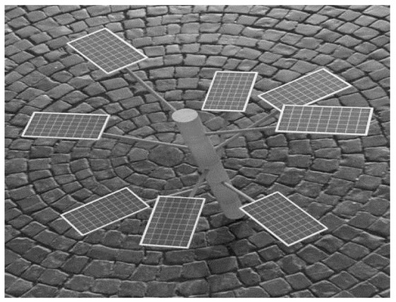
Verma NN, Mazumder S (2015) An investigation of solar trees for effective sunlight capture using monte carlo simulations of solar radiation transport. ASME 2014 International Mechanical Engineering Congress and Exposition. https://doi.org/10.1115/IMECE2014-36085 doi: 10.1115/IMECE2014-36085
![]() |
[127] |
Gangwar P, Kumar NM, Singh AK, et al. (2019) Solar photovoltaic tree and its end-of-life management using thermal and chemical treatments for material recovery. Case Stud Therm Eng 14: 100474. https://doi.org/10.1016/J.CSITE.2019.100474 doi: 10.1016/j.csite.2019.100474
![]() |
[128] | Mostafaeipour A, Rezaei M, Jahangiri M, et al. (2019) Feasibility analysis of a new tree-shaped wind turbine for urban application: A case study. 31: 1230–1256. https://doi.org/101177/0958305X19888878 |
[129] |
Berny S, Blouin N, Distler A, et al. (2016) Solar trees: First large-scale demonstration of fully solution coated, semitransparent, flexible organic photovoltaic modules. Adv Sci 3: 1500342. https://doi.org/10.1016/J.CSITE.2019.100474 doi: 10.1002/advs.201500342
![]() |
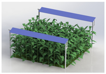
[130] | Perna A, Grubbs EK, Agrawal R, et al. (2019) Design considerations for Agrophotovoltaic systems: Maintaining PV area with increased crop yield. Conference Record of the IEEE Photovoltaic Specialists Conference Institute of Electrical and Electronics Engineers Inc., 668–672. https://doi.org/10.1109/PVSC40753.2019.8981324 |
[131] |
Amaducci S, Yin X, Colauzzi M (2018) Agrivoltaic systems to optimise land use for electric energy production. Appl Energy 220: 545–561. https://doi.org/10.1016/j.apenergy.2018.03.081 doi: 10.1016/j.apenergy.2018.03.081
![]() |
[132] | Weselek A, Ehmann A, Zikeli S, et al. (2019) Agrophotovoltaic systems: applications, challenges, and opportunities. A review. Agron Sustainable Dev 39: 1–20. Available from: https://link.springer.com/article/10.1007/s13593-019-0581-3. |
[133] |
Schindele S, Trommsdorff M, Schlaak A, et al. (2020) Implementation of agrophotovoltaics: Techno-economic analysis of the price-performance ratio and its policy implications. Appl Energy 265: 114737. https://doi.org/10.1016/J.APENERGY.2020.114737 doi: 10.1016/j.apenergy.2020.114737
![]() |
[134] | IEA (2019) The future of hydrogen, Paris. Available from: https://www.iea.org/reports/the-future-of-hydrogen#. |
[135] |
Han Y, Pu Y, Li Q, et al. (2019) Coordinated power control with virtual inertia for fuel cell-based DC microgrids cluster. Int J Hydrogen Energy 44: 25207–25220. https://doi.org/10.1016/J.IJHYDENE.2019.06.128 doi: 10.1016/j.ijhydene.2019.06.128
![]() |
[136] |
Tostado-Véliz M, Kamel S, Hasanien HM, et al. (2022) A mixed-integer-linear-logical programming interval-based model for optimal scheduling of isolated microgrids with green hydrogen-based storage considering demand response. J Energy Storage 48: 104028. https://doi.org/10.1016/J.EST.2022.104028 doi: 10.1016/j.est.2022.104028
![]() |
× | 0 | a | b | c |
0 | 0 | 0 | 0 | 0 |
a | 0 | b | 0 | b |
b | 0 | 0 | 0 | 0 |
c | 0 | b | 0 | b |
× | 0 | a | b | c |
0 | 0 | 0 | 0 | 0 |
a | 0 | a | a | 0 |
b | 0 | b | b | 0 |
c | 0 | c | c | 0 |
r | s | t | u | CPI(r,s,t,u) is QSD |
{0,b} | {0,b} | {0,b} | {0,b} | never |
{0,b} | {0,b} | {0,b} | {a,c} | n≡0 and β≡λ |
{0,b} | {0,b} | {a,c} | {0,b} | κ+1≡λ≡μ≡0 |
{0,b} | {0,b} | {a,c} | {a,c} | κ≡λ+1≡μ≡n |
{0,b} | {a,c} | {0,b} | {0,b} | κ+1≡λ≡μ≡0 |
{0,b} | {a,c} | {0,b} | {a,c} | κ≡λ+1≡μ≡n |
{0,b} | {a,c} | {a,c} | {0,b} | never |
{0,b} | {a,c} | {a,c} | {a,c} | n≡0 |
{a,c} | {0,b} | {0,b} | {0,b} | always |
{a,c} | {0,b} | {0,b} | {a,c} | never |
{a,c} | {0,b} | {a,c} | {0,b} | κ≡λ+1≡μ≡0 |
{a,c} | {0,b} | {a,c} | {a,c} | κ+1≡λ≡μ≡n |
{a,c} | {a,c} | {0,b} | {0,b} | κ≡λ+1≡μ≡0 |
{a,c} | {a,c} | {0,b} | {a,c} | κ+1≡λ≡μ≡n |
{a,c} | {a,c} | {a,c} | {0,b} | β≡λ |
{a,c} | {a,c} | {a,c} | {a,c} | never |
r | s | t | u | CBI(r,s,t,u) is QSD |
{0,b} | {0,b} | {0,b} | {0,b} | never |
{0,b} | {0,b} | {0,b} | {a,c} | n≡1 and β≡λ |
{0,b} | {0,b} | {a,c} | {0,b} | κ+1≡λ≡μ≡n≡1 |
{0,b} | {0,b} | {a,c} | {a,c} | κ≡λ+1≡μ≡n+1≡0 |
{0,b} | {a,c} | {0,b} | {0,b} | κ+1≡λ≡μ≡n≡1 |
{0,b} | {a,c} | {0,b} | {a,c} | κ≡λ+1≡μ≡n+1≡0 |
{0,b} | {a,c} | {a,c} | {0,b} | never |
{0,b} | {a,c} | {a,c} | {a,c} | n≡1 |
{a,c} | {0,b} | {0,b} | {0,b} | never |
{a,c} | {0,b} | {0,b} | {a,c} | never |
{a,c} | {0,b} | {a,c} | {0,b} | κ≡λ+1≡μ≡n≡1 |
{a,c} | {0,b} | {a,c} | {a,c} | κ+1≡λ≡μ≡n+1≡0 |
{a,c} | {a,c} | {0,b} | {0,b} | κ≡λ+1≡μ≡n≡1 |
{a,c} | {a,c} | {0,b} | {a,c} | κ+1≡λ≡μ≡n+1≡0 |
{a,c} | {a,c} | {a,c} | {0,b} | never |
{a,c} | {a,c} | {a,c} | {a,c} | never |
Construction | (n,κ,β,λ,μ) | Code | (N,d) | Type Ⅳ |
(6,1,1,0,0) | CPI(a,0,a,a) | (12,4) | yes | |
(9,1,1,0,0) | CPI(a,b,b,0) | (18,2) | yes | |
(12,1,1,0,0) | CPI(b,a,a,a) | (24,4) | no | |
(14,3,2,1,0) | CPI(0,a,a,a) | (28,4) | yes | |
(15,1,1,0,0) | CPI(0,a,0,b) | (30,2) | yes | |
Pure | (18,1,1,0,0) | CPI(0,a,c,c) | (36,4) | no |
(21,3,2,1,0) | CPI(a,0,0,b) | (42,2) | yes | |
(22,5,3,2,0) | CPI(c,0,c,a) | (44,8) | yes | |
(28,3,2,1,0) | CPI(0,a,a,a) | (56,4) | yes | |
(33,5,3,2,0) | CPI(0,0,a,0) | (66,6) | yes | |
(38,9,5,4,0) | CPI(c,c,0,c) | (76,8) | yes | |
(9,1,1,0,0) | CBI(0,c,c,a) | (20,4) | yes | |
Bordered | (15,1,1,0,0) | CBI(0,a,a,a) | (32,4) | yes |
(33,5,3,2,0) | CBI(c,0,c,a) | (68,8) | yes |
r | s | t | u | CPI(r,s,t,u) is QSD |
{0,b} | {0,b} | {0,b} | {0,b} | never |
{0,b} | {0,b} | {0,b} | {a,c} | α1+α2≡β1+β2≡γ1+γ2≡κ1+κ2≡n |
{0,b} | {0,b} | {a,c} | {0,b} | α2≡β2≡γ2≡κ2+1≡0 |
{0,b} | {0,b} | {a,c} | {a,c} | α1≡β1≡γ1≡κ1≡n |
{0,b} | {a,c} | {0,b} | {0,b} | α1≡β1≡γ1≡κ1+1≡0 |
{0,b} | {a,c} | {0,b} | {a,c} | α2≡β2≡γ2≡κ2≡n |
{0,b} | {a,c} | {a,c} | {0,b} | α1+α2≡β1+β2≡γ1+γ2≡κ1+κ2+1≡0 |
{0,b} | {a,c} | {a,c} | {a,c} | n≡0 |
{a,c} | {0,b} | {0,b} | {0,b} | always |
{a,c} | {0,b} | {0,b} | {a,c} | α1+α2≡β1+β2≡γ1+γ2≡κ1+κ2+1≡n |
{a,c} | {0,b} | {a,c} | {0,b} | α2≡β2≡γ2≡κ2≡0 |
{a,c} | {0,b} | {a,c} | {a,c} | α1≡β1≡γ1≡κ1+1≡n |
{a,c} | {a,c} | {0,b} | {0,b} | α1≡β1≡γ1≡κ1≡0 |
{a,c} | {a,c} | {0,b} | {a,c} | α2≡β2≡γ2≡κ2+1≡n |
{a,c} | {a,c} | {a,c} | {0,b} | α1+α2≡β1+β2≡γ1+γ2≡κ1+κ2≡0 |
{a,c} | {a,c} | {a,c} | {a,c} | never |
r | s | t | u | CBI(r,s,t,u) is QSD |
{0,b} | {0,b} | {0,b} | {0,b} | never |
{0,b} | {0,b} | {0,b} | {a,c} | α1+α2≡β1+β2≡γ1+γ2≡n+1≡0 |
{0,b} | {0,b} | {a,c} | {0,b} | α2≡β2≡γ2≡n≡1 |
{0,b} | {0,b} | {a,c} | {a,c} | α1≡β1≡γ1≡n+1≡0 |
{0,b} | {a,c} | {0,b} | {0,b} | α1≡β1≡γ1≡n≡1 |
{0,b} | {a,c} | {0,b} | {a,c} | α2≡β2≡γ2≡n+1≡0 |
{0,b} | {a,c} | {a,c} | {0,b} | α1+α2≡β1+β2≡γ1+γ2≡n≡1 |
{0,b} | {a,c} | {a,c} | {a,c} | n≡1 |
{a,c} | I | I | I | never |
r | s | t | u | CPI(r,s,t,u) is Type Ⅳ |
≠ | ≠ | ≠ | b | n≡κ1+κ2+1 |
≠ | ≠ | b | ≠ | κ2≡0 |
≠ | ≠ | b | b | n≡κ1+1 |
≠ | b | ≠ | ≠ | κ1≡0 |
≠ | b | ≠ | b | n≡κ2+1 |
≠ | b | b | ≠ | κ1≡κ2 |
≠ | b | b | b | n≡1 |
b | ≠ | ≠ | ≠ | never |
b | ≠ | ≠ | b | n≡κ1+κ2 |
b | ≠ | b | ≠ | κ2≡1 |
b | ≠ | b | b | n≡κ1 |
b | b | ≠ | ≠ | κ1≡1 |
b | b | ≠ | b | n≡κ2 |
b | b | b | ≠ | κ1+κ2≡1 |
r | s | t | u | wt(gi) (mod 2) |
≠ | ≠ | ≠ | ≠ | 0 |
≠ | ≠ | ≠ | b | n+κ1+κ2+1 |
≠ | ≠ | b | ≠ | κ2 |
≠ | ≠ | b | b | n+κ1+1 |
≠ | b | ≠ | ≠ | κ1 |
≠ | b | ≠ | b | n+κ2+1 |
≠ | b | b | ≠ | κ1+κ2 |
≠ | b | b | b | n+1 |
b | ≠ | ≠ | ≠ | 1 |
b | ≠ | ≠ | b | n+κ1+κ2 |
b | ≠ | b | ≠ | κ2+1 |
b | ≠ | b | b | n+κ1 |
b | b | ≠ | ≠ | κ1+1 |
b | b | ≠ | b | n+κ2 |
b | b | b | ≠ | κ1+κ2+1 |
Construction | (n,κ1,κ2) | Code | (N,d) | Type Ⅳ |
(6,1,2) | CPI(a,0,a,a) | (12,4) | yes | |
(7,2,2) | CPI(a,0,0,0) | (14,2) | yes | |
(9,2,2) | CPI(a,b,0,b) | (18,2) | yes | |
(10,2,2) | CPI(b,a,a,a) | (20,4) | no | |
(12,1,5) | CPI(b,0,a,b) | (24,4) | yes | |
Pure | (14,3,4) | CPI(a,0,a,0) | (28,6) | yes |
(16,3,3) | CPI(0,a,b,0) | (32,4) | no | |
(18,2,4) | CPI(c,c,0,c) | (36,4) | yes | |
(26,4,9) | CPI(a,a,0,a) | (52,8) | yes | |
(28,3,12) | CPI(b,a,b,a) | (56,8) | no | |
(32,6,10) | CPI(a,b,a,0) | (64,8) | yes | |
(7,2,2) | CBI(0,a,a,a) | (16,4) | yes | |
(9,2,2) | CBI(0,a,c,a) | (20,4) | yes | |
(15,2,4) | CBI(0,c,a,b) | (32,8) | yes | |
Bordered | (19,6,6) | CBI(b,a,a,a) | (40,4) | no |
(21,4,8) | CBI(0,a,b,c) | (44,8) | yes | |
(27,2,8) | CBI(0,c,a,0) | (56,8) | yes | |
(33,2,10) | CBI(0,c,c,c) | (68,4) | yes |
× | 0 | a | b | c |
0 | 0 | 0 | 0 | 0 |
a | 0 | b | 0 | b |
b | 0 | 0 | 0 | 0 |
c | 0 | b | 0 | b |
× | 0 | a | b | c |
0 | 0 | 0 | 0 | 0 |
a | 0 | a | a | 0 |
b | 0 | b | b | 0 |
c | 0 | c | c | 0 |
r | s | t | u | CPI(r,s,t,u) is QSD |
{0,b} | {0,b} | {0,b} | {0,b} | never |
{0,b} | {0,b} | {0,b} | {a,c} | n≡0 and β≡λ |
{0,b} | {0,b} | {a,c} | {0,b} | κ+1≡λ≡μ≡0 |
{0,b} | {0,b} | {a,c} | {a,c} | κ≡λ+1≡μ≡n |
{0,b} | {a,c} | {0,b} | {0,b} | κ+1≡λ≡μ≡0 |
{0,b} | {a,c} | {0,b} | {a,c} | κ≡λ+1≡μ≡n |
{0,b} | {a,c} | {a,c} | {0,b} | never |
{0,b} | {a,c} | {a,c} | {a,c} | n≡0 |
{a,c} | {0,b} | {0,b} | {0,b} | always |
{a,c} | {0,b} | {0,b} | {a,c} | never |
{a,c} | {0,b} | {a,c} | {0,b} | κ≡λ+1≡μ≡0 |
{a,c} | {0,b} | {a,c} | {a,c} | κ+1≡λ≡μ≡n |
{a,c} | {a,c} | {0,b} | {0,b} | κ≡λ+1≡μ≡0 |
{a,c} | {a,c} | {0,b} | {a,c} | κ+1≡λ≡μ≡n |
{a,c} | {a,c} | {a,c} | {0,b} | β≡λ |
{a,c} | {a,c} | {a,c} | {a,c} | never |
r | s | t | u | CBI(r,s,t,u) is QSD |
{0,b} | {0,b} | {0,b} | {0,b} | never |
{0,b} | {0,b} | {0,b} | {a,c} | n≡1 and β≡λ |
{0,b} | {0,b} | {a,c} | {0,b} | κ+1≡λ≡μ≡n≡1 |
{0,b} | {0,b} | {a,c} | {a,c} | κ≡λ+1≡μ≡n+1≡0 |
{0,b} | {a,c} | {0,b} | {0,b} | κ+1≡λ≡μ≡n≡1 |
{0,b} | {a,c} | {0,b} | {a,c} | κ≡λ+1≡μ≡n+1≡0 |
{0,b} | {a,c} | {a,c} | {0,b} | never |
{0,b} | {a,c} | {a,c} | {a,c} | n≡1 |
{a,c} | {0,b} | {0,b} | {0,b} | never |
{a,c} | {0,b} | {0,b} | {a,c} | never |
{a,c} | {0,b} | {a,c} | {0,b} | κ≡λ+1≡μ≡n≡1 |
{a,c} | {0,b} | {a,c} | {a,c} | κ+1≡λ≡μ≡n+1≡0 |
{a,c} | {a,c} | {0,b} | {0,b} | κ≡λ+1≡μ≡n≡1 |
{a,c} | {a,c} | {0,b} | {a,c} | κ+1≡λ≡μ≡n+1≡0 |
{a,c} | {a,c} | {a,c} | {0,b} | never |
{a,c} | {a,c} | {a,c} | {a,c} | never |
Construction | (n,κ,β,λ,μ) | Code | (N,d) | Type Ⅳ |
(6,1,1,0,0) | CPI(a,0,a,a) | (12,4) | yes | |
(9,1,1,0,0) | CPI(a,b,b,0) | (18,2) | yes | |
(12,1,1,0,0) | CPI(b,a,a,a) | (24,4) | no | |
(14,3,2,1,0) | CPI(0,a,a,a) | (28,4) | yes | |
(15,1,1,0,0) | CPI(0,a,0,b) | (30,2) | yes | |
Pure | (18,1,1,0,0) | CPI(0,a,c,c) | (36,4) | no |
(21,3,2,1,0) | CPI(a,0,0,b) | (42,2) | yes | |
(22,5,3,2,0) | CPI(c,0,c,a) | (44,8) | yes | |
(28,3,2,1,0) | CPI(0,a,a,a) | (56,4) | yes | |
(33,5,3,2,0) | CPI(0,0,a,0) | (66,6) | yes | |
(38,9,5,4,0) | CPI(c,c,0,c) | (76,8) | yes | |
(9,1,1,0,0) | CBI(0,c,c,a) | (20,4) | yes | |
Bordered | (15,1,1,0,0) | CBI(0,a,a,a) | (32,4) | yes |
(33,5,3,2,0) | CBI(c,0,c,a) | (68,8) | yes |
r | s | t | u | CPI(r,s,t,u) is QSD |
{0,b} | {0,b} | {0,b} | {0,b} | never |
{0,b} | {0,b} | {0,b} | {a,c} | α1+α2≡β1+β2≡γ1+γ2≡κ1+κ2≡n |
{0,b} | {0,b} | {a,c} | {0,b} | α2≡β2≡γ2≡κ2+1≡0 |
{0,b} | {0,b} | {a,c} | {a,c} | α1≡β1≡γ1≡κ1≡n |
{0,b} | {a,c} | {0,b} | {0,b} | α1≡β1≡γ1≡κ1+1≡0 |
{0,b} | {a,c} | {0,b} | {a,c} | α2≡β2≡γ2≡κ2≡n |
{0,b} | {a,c} | {a,c} | {0,b} | α1+α2≡β1+β2≡γ1+γ2≡κ1+κ2+1≡0 |
{0,b} | {a,c} | {a,c} | {a,c} | n≡0 |
{a,c} | {0,b} | {0,b} | {0,b} | always |
{a,c} | {0,b} | {0,b} | {a,c} | α1+α2≡β1+β2≡γ1+γ2≡κ1+κ2+1≡n |
{a,c} | {0,b} | {a,c} | {0,b} | α2≡β2≡γ2≡κ2≡0 |
{a,c} | {0,b} | {a,c} | {a,c} | α1≡β1≡γ1≡κ1+1≡n |
{a,c} | {a,c} | {0,b} | {0,b} | α1≡β1≡γ1≡κ1≡0 |
{a,c} | {a,c} | {0,b} | {a,c} | α2≡β2≡γ2≡κ2+1≡n |
{a,c} | {a,c} | {a,c} | {0,b} | α1+α2≡β1+β2≡γ1+γ2≡κ1+κ2≡0 |
{a,c} | {a,c} | {a,c} | {a,c} | never |
r | s | t | u | CBI(r,s,t,u) is QSD |
{0,b} | {0,b} | {0,b} | {0,b} | never |
{0,b} | {0,b} | {0,b} | {a,c} | α1+α2≡β1+β2≡γ1+γ2≡n+1≡0 |
{0,b} | {0,b} | {a,c} | {0,b} | α2≡β2≡γ2≡n≡1 |
{0,b} | {0,b} | {a,c} | {a,c} | α1≡β1≡γ1≡n+1≡0 |
{0,b} | {a,c} | {0,b} | {0,b} | α1≡β1≡γ1≡n≡1 |
{0,b} | {a,c} | {0,b} | {a,c} | α2≡β2≡γ2≡n+1≡0 |
{0,b} | {a,c} | {a,c} | {0,b} | α1+α2≡β1+β2≡γ1+γ2≡n≡1 |
{0,b} | {a,c} | {a,c} | {a,c} | n≡1 |
{a,c} | I | I | I | never |
r | s | t | u | CPI(r,s,t,u) is Type Ⅳ |
≠ | ≠ | ≠ | b | n≡κ1+κ2+1 |
≠ | ≠ | b | ≠ | κ2≡0 |
≠ | ≠ | b | b | n≡κ1+1 |
≠ | b | ≠ | ≠ | κ1≡0 |
≠ | b | ≠ | b | n≡κ2+1 |
≠ | b | b | ≠ | κ1≡κ2 |
≠ | b | b | b | n≡1 |
b | ≠ | ≠ | ≠ | never |
b | ≠ | ≠ | b | n≡κ1+κ2 |
b | ≠ | b | ≠ | κ2≡1 |
b | ≠ | b | b | n≡κ1 |
b | b | ≠ | ≠ | κ1≡1 |
b | b | ≠ | b | n≡κ2 |
b | b | b | ≠ | κ1+κ2≡1 |
r | s | t | u | wt(gi) (mod 2) |
≠ | ≠ | ≠ | ≠ | 0 |
≠ | ≠ | ≠ | b | n+κ1+κ2+1 |
≠ | ≠ | b | ≠ | κ2 |
≠ | ≠ | b | b | n+κ1+1 |
≠ | b | ≠ | ≠ | κ1 |
≠ | b | ≠ | b | n+κ2+1 |
≠ | b | b | ≠ | κ1+κ2 |
≠ | b | b | b | n+1 |
b | ≠ | ≠ | ≠ | 1 |
b | ≠ | ≠ | b | n+κ1+κ2 |
b | ≠ | b | ≠ | κ2+1 |
b | ≠ | b | b | n+κ1 |
b | b | ≠ | ≠ | κ1+1 |
b | b | ≠ | b | n+κ2 |
b | b | b | ≠ | κ1+κ2+1 |
Construction | (n,κ1,κ2) | Code | (N,d) | Type Ⅳ |
(6,1,2) | CPI(a,0,a,a) | (12,4) | yes | |
(7,2,2) | CPI(a,0,0,0) | (14,2) | yes | |
(9,2,2) | CPI(a,b,0,b) | (18,2) | yes | |
(10,2,2) | CPI(b,a,a,a) | (20,4) | no | |
(12,1,5) | CPI(b,0,a,b) | (24,4) | yes | |
Pure | (14,3,4) | CPI(a,0,a,0) | (28,6) | yes |
(16,3,3) | CPI(0,a,b,0) | (32,4) | no | |
(18,2,4) | CPI(c,c,0,c) | (36,4) | yes | |
(26,4,9) | CPI(a,a,0,a) | (52,8) | yes | |
(28,3,12) | CPI(b,a,b,a) | (56,8) | no | |
(32,6,10) | CPI(a,b,a,0) | (64,8) | yes | |
(7,2,2) | CBI(0,a,a,a) | (16,4) | yes | |
(9,2,2) | CBI(0,a,c,a) | (20,4) | yes | |
(15,2,4) | CBI(0,c,a,b) | (32,8) | yes | |
Bordered | (19,6,6) | CBI(b,a,a,a) | (40,4) | no |
(21,4,8) | CBI(0,a,b,c) | (44,8) | yes | |
(27,2,8) | CBI(0,c,a,0) | (56,8) | yes | |
(33,2,10) | CBI(0,c,c,c) | (68,4) | yes |