Classification, prioritization, efficiency, and change management of EPC projects in Energy and Petroleum industry field using the TOPSIS method as a multi-criteria group decision-making method

1.   Introduction

A molecular graph is a graph such that its vertices correspond to the atoms and the edges to the bonds. Chemical Graph Theory is a branch of Mathematical Chemistry, which has an important effect on the development of the Chemical Sciences. A topological index is a numerical parameter mathematically derived from the graph structure. Several such topological indices have been considered in Theoretical Chemistry and have found some applications, especially in QSPR/QSAR study see ^[1,2].

Let $G$ be a finite, simple, connected graph with vertex set $V(G)$ and edge set $E(G)$. The degree $d_G(u)$ of a vertex $u$ is the number of vertices adjacent to $u$. Let $\Delta (G)$ and $\delta (G)$ denote the maximum and minimum degree, respectively, among the vertices of $G$. The Revan vertex degree of a vertex $u \in V(G)$ is defined as $r_G(u) = \Delta(G) + \delta(G) - d_G(u)$. The edge connecting the vertices $u, v \in V(G)$ will be denoted by $uv$. We refer to ^[3] for undefined notations and terminologies.

The first and second Revan indices of a graph $G$ were introduced by Kulli in ^[4], and they are defined as

The $F$-Revan index of a graph is defined in ^[5] as

The Sombor index was introduced by Gutman in ^[6], defined as

Recently, a large number of studies on Sombor indices have been published, see e.g., ^{[7,8,9,10,11,12,13,14,15]}.

The Revan Sombor index was proposed by Kulli and Gutman in ^[16] as

The first and second Revan $(a, b)$-$KA$ indices of a graph $G$ are defined (generalizing the Revan Sombor index), respectively, as

Recently, some $(a, b)$-KA indices have been used to analyze the properties of chemical compounds and nanostructures. In particular, they have been applied to the study of benzenoid systems and phenylenes, see for example ^{[17,18,19,20]}.

Therefore, motivated both by their practical applications as well as by their theoretical properties, mainly because of the close relationship with the well-known Sombor index ^[15], in this paper we perform analytical and statistical studies on the recently introduced Revan Sombor indices.

2.   Inequalities for the Revan Sombor index

Theorem 1. If $G$ is a graph with maximum degree $\Delta$ and minimum degree $\delta$, and $c \in \mathbb{R} \setminus \{0\}$, then

and the equality in each bound is attained for each $c$ if and only if $G$ is a regular graph.

Proof. If $c > 0$, then

and we obtain the converse inequality if $c < 0$. The equality in each bound is attained if and only if $r_G(u) = r_G(v) = \Delta$, i.e., $d_G(u) = d_G(v) = \delta$ for every $uv \in E(G)$, that is, $G$ is a regular graph.

Also, if $c > 0$, then

and we obtain the converse inequality if $c < 0$. The equality in each bound is attained if and only if $r_G(u) = r_G(v) = \delta$, i.e., $d_G(u) = d_G(v) = \Delta$ for every $uv \in E(G)$, that is, $G$ is a regular graph.

Notice that the limit as $c$ approaches zero, the bounds, both upper and lower, are all equal to $m$ (number of edges of $G$).

If we choose $c = 1$ in Theorem 1, then we obtain the following result.

Corollary 2. If $G$ is a graph, then

and the equality in each bound is attained if and only if $G$ is a regular graph.

Theorem 3. If $G$ is a graph with $m$ edges and maximum degree $\Delta$, and $c > 0$, then

and the equality in the bound is attained for each $c$ if and only if $G$ is a regular graph.

Proof. Cauchy-Schwarz inequality gives

If the equality in the bound is attained for some $c > 0$, then $r_G(u) = r_G(v) = \Delta$ for every $uv \in E(G)$ and so, $G$ is a regular graph.

If $G$ is regular, then

If we choose $c = 1$ in Theorem 3, then we obtain the following result.

Corollary 4. If $G$ is a graph with $m$ edges and maximum degree $\Delta$, then

and the equality in the bound is attained if and only if $G$ is a regular graph.

We need the following well known inequalities for $x_1, x_2 > 0$ ^[21]:

and the equality in each non-strict inequality is attained for each $\alpha$ if and only if $x_1 = x_2$.

These inequalities allow to obtain the following result.

Theorem 5. If $G$ is a graph and $a, b, c \in \mathbb{R} \setminus \{0\}$, then

and the equality in each non-strict inequality is attained for each $a, b, c$ if and only if each connected component of $G$ is a regular graph.

Proof. If $\alpha = b/c$, $x_1 = r_G(u)^{a}$ and $x_2 = r_G(v)^{a}$, then the previous inequalities give

and the equality in each non-strict inequality is attained if and only if $r_G(u) = r_G(v)$, i.e., $d_G(u) = d_G(v)$.

Hence, we obtain

and the equality in each non-strict inequality is attained if and only if $d_G(u) = d_G(v)$.

If we sum on $uv \in E(G)$ these inequalities, then we obtain the desired inequalities. Furthermore, the equality in each non-strict inequality is attained for each $a, b, c$ if and only if $d_G(u) = d_G(v)$ for every $uv \in E(G)$; and this happens if and only if each connected component of $G$ is a regular graph.

Remark 6. The excluded case $b = c$ in Theorem 5 is not interesting, since $RK\!A^1_{ab/c, \, c}(G) = RK\!A^1_{a, b}(G)$ if $b = c$.

If we take $a = 2$, $b = 1/2$ and $c = 1/ \alpha$ in Theorem 5, then we obtain the following result for the Revan Sombor index.

Corollary 7. If $G$ is a graph and $\alpha \in \mathbb{R} \setminus \{0\}$, then

and the equality in each non-strict inequality is attained for each $\alpha$ if and only if each connected component of $G$ is a regular graph.

The above bounds (in Theorem 5 and Corollary 7) are achieved for several families of graphs, e.g., the complete graph $K_n$, the complete bipartite graph $K_{m, n}$, the cycle graph $C_n$, etc.

Recall that one of the most studied topological indices is the first Zagreb index, defined by

Our next result relates $M_1$ and $RK\!A^1_{ \alpha, \, 1/ \alpha}$.

Theorem 8. If $G$ is a graph with $m$ edges, maximum degree $\Delta$ and minimum degree $\delta$, and $\alpha \in \mathbb{R} \setminus \{0\}$, then

and the equality in each non-strict inequality is attained for each $\alpha$ if and only if each connected component of $G$ is a regular graph.

Proof. If we take $a = b = 1$ and $c = 1/ \alpha$ in Theorem 5, then we obtain the following result for $RK\!A^1_{1, 1}(G)$:

and the equality in each non-strict inequality is attained for each $\alpha$ if and only if each connected component of $G$ is a regular graph.

These inequalities and the identity

finish the proof.

The first and second $(a, b)$-$KA$ indices of a graph $G$ are defined in ^[17], respectively, as

The following result relates the $K\!A^1_{a, \, b}$ and $RK\!A^1_{a, \, b}$ indices.

Theorem 9. If $G$ is a graph with maximum degree $\Delta$ and minimum degree $\delta$, and $a, b \in \mathbb{R} \setminus \{0\}$, then

and the equality in each inequality is attained for each $a, b$ if and only if $G$ is a regular graph.

Proof. Let us define the function $f: [\delta, \Delta]\times [\delta, \Delta] \rightarrow (0, \infty)$ by

Note that if $a > 0$, the numerator of $f$ is strictly decreasing on $[\delta, \Delta]$ on each variable and its denominator is strictly increasing on $[\delta, \Delta]$ on each variable. Hence, $f$ is a strictly decreasing function on $[\delta, \Delta]$ on each variable, and so,

If $x = d_G(u)$ and $y = d_G(v)$, then

Notice that if $b > 0$, then the above inequality is preserved; thus

In contrast, if $b < 0$, then the inequality above is not preserved; thus

If $a < 0$, then $f$ is a strictly increasing function on $[\delta, \Delta]$ on each variable, and so,

Thus,

if $b < 0$, and

if $b > 0$.

If we sum on $uv \in E(G)$ these inequalities, then we obtain the desired inequalities. Furthermore, since $f$ is a strictly monotone function, the equality in each inequality is attained for each $a, b$ if and only if $d_G(u) = d_G(v) = \delta$ for every $uv \in E(G)$ or $d_G(u) = d_G(v) = \Delta$ for every $uv \in E(G)$; and this happens if and only if $G$ is a regular graph.

The Revan Sombor and the Sombor indices have the same value for every regular graph. The following result, which is a consequence of Theorem 9 with $a = 2$ and $b = 1/2$, relates these two indices for every graph.

Corollary 10. If $G$ is a graph with maximum degree $\Delta$ and minimum degree $\delta$, then

and the equality in each inequality is attained if and only if $G$ is a regular graph.

Another remarkable topological index is the harmonic index, defined in ^[22] as

This index has attracted a great interest in the lasts years (see, e.g., ^{[23,24,25,26,27]}).

The next result relates the $RK\!A^1_{a, \, 1/a}$ and the harmonic indices.

Theorem 11. If $G$ is a graph with maximum degree $\Delta$ and minimum degree $\delta$, and $a \in \mathbb{R}$, then

The equality in the first inequality is attained for each $a$ if and only if each connected component of $G$ is $\Delta$-regular or $\delta$-regular. The equality in the two last inequalities is attained for each $a$ if $G$ is a regular graph.

Proof. Recall that

for $x_1, x_2 > 0$, and the equality in each non-strict inequality is attained for each $a$ if and only if $x_1 = x_2$.

Let us define the function $g: [\delta, \Delta]\times [\delta, \Delta] \rightarrow (0, \infty)$ by

If $a > 1$, then

since $x+y \in [2 \delta, 2 \Delta]$. Thus,

for every $uv \in E(G)$, and so,

Also,

since $x+y \in [2 \delta, 2 \Delta]$. The equality in the previous bound is attained if and only if we have either $x = y = \delta$ or $x = y = \Delta$. Therefore,

for every $uv \in E(G)$, and so,

The equality in this bound is attained for each $a > 1$ if and only if for each edge $uv \in E(G)$ we have either $d_G(u) = d_G(v) = \Delta$ or $d_G(u) = d_G(v) = \delta$, that is, each connected component of $G$ is $\Delta$-regular or $\delta$-regular.

Assume now $a < 1$, then

since $x+y \in [2 \delta, 2 \Delta]$. Thus,

for every $uv \in E(G)$, and so,

If $G$ is a regular graph with $m$ edges, then

If $0 < a < 1$, then we have

since $x+y \in [2 \delta, 2 \Delta]$. Therefore,

for every $uv \in E(G)$, and so,

If we choose $a = 2$ in Theorem 11, then we obtain the following result for the Revan Sombor index.

Corollary 12. If $G$ is a graph with maximum degree $\Delta$ and minimum degree $\delta$, then

and the equality in the first inequality is attained if and only if each connected component of $G$ is $\Delta$-regular or $\delta$-regular.

3.   Revan Sombor indices on random graphs

Recently, within a statistical approach to degree-based topological indices (TIs) on random graphs (see e.g., ^[28,29,30]), it has been shown that the average values of TIs like the average Randic index, $\langle R(G) \rangle$, the average harmonic index, $\langle H(G) \rangle$, and the average of some Sombor indices are highly correlated with the average Shannon entropy of the eigenvectors of the corresponding adjacency matrix ^[31,32]. Here, $\left < \cdot \right >$ denotes the average over an ensemble of random graphs. This is a notable result because it puts forward the application of degree-based TIs beyond mathematical chemistry (it is relevant to add that random graphs have also been studied by means of eigenvalue-based TIs such as the Estrada index, the Laplacian Estrada index, and Rodriguez-Velazquez indices, see e.g., ^[33,34].) Specifically, on the one hand, certain average TIs can provide equivalent information than traditional, spectrum-based, random matrix theory measures. On the other hand, TIs may be used to predict spectral properties of random graphs.

Therefore, motivated by potential applications, in what follows we apply for the first time (to our knowledge) Revan degree-based indices on random graphs. Indeed, since the inequalities obtained in Section 2 are not restricted to any particular type of graph, we first quantify them for random graphs and later we extend some of them to index average values, as needed in statistical studies of random graphs.

Below we consider two prominent models of random graphs: Erdös-Rényi (ER) graphs and random geometric (RG) graphs. ER graphs ^[35,36] $G_{\mbox{ER}}(n, p)$ are formed by $n$ vertices connected independently with probability $p \in [0, 1]$. While RG graphs ^[37,38] $G_{\mbox{RG}}(n, r)$ consist of $n$ vertices uniformly and independently distributed on the unit square, where two vertices are connected by an edge if their Euclidean distance is less or equal than the connection radius $r \in [0, \sqrt{2}]$.

3.1.   Quantification of inequalities for random graphs

In the Theorems presented in Section 2 we know the graph properties needed for the equalities involved have to be attained, however we do not really know how strong the inequalities could be for arbitrary graphs. Thus, in this subsection we quantify the inequalities of those Theorems on random graphs.

To ease the quantification of the six Theorems presented in Section 2 we:

$\rm(i)$ write the left inequality of Corollary 2 as

$\rm(ii)$ write Corollary 4 as

$\rm(iii)$ write the right inequality in the second line of Corollary 7, for $\alpha = 1/2$, as

$\rm(iv)$ write the left inequality in the second line of Theorem 8, for $\alpha = 1/2$, as

$\rm(v)$ write the left inequality of Corollary 10 as

and

$\rm(vi)$ write the left inequality of Corollary 12 as

Then, in Figure 1 [in Figure 2] we plot the right hand side of Eqs (3.1)–(3.6) as a function of the probability $p$ [the connection radius $r$] of ER [RG] graphs of size $n$. For each value of $p$ [$r$] we present results for 10 graph realizations.

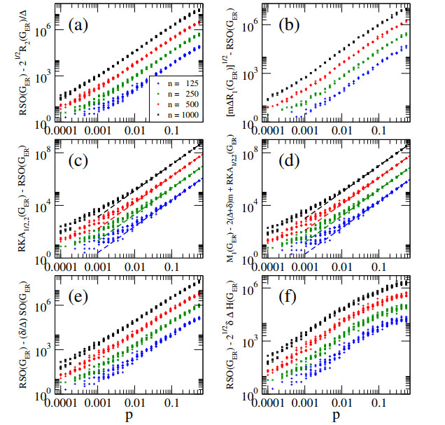
Figure 1.  Right hand side of (a) Eq (3.1), (b) Eq (3.2), (c) Eq (3.3), (d) Eq (3.4), (e) Eq (3.5) and (f) Eq (3.6) as a function of the probability $p$ of Erdős-Rényi graphs $G_{\mbox{ER}}(n, p)$ of size $n$. Each symbol corresponds to a single graph realization. Dashed lines in (c) [(d)] correspond to Eq (3.7) [(3.8)] with $\langle d_G \rangle = (n-1)p$.

DownLoad: Full-Size Img PowerPoint

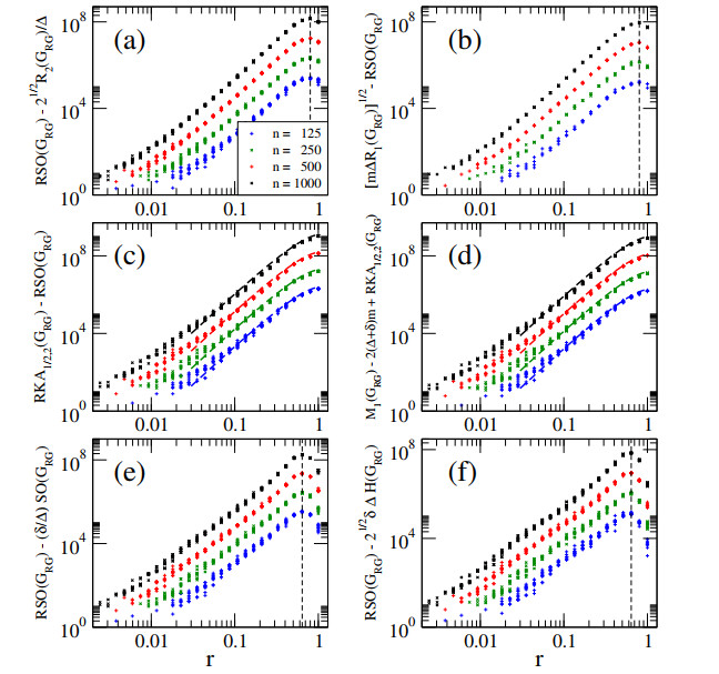
Figure 2.  Right hand side of (a) Eq (3.1), (b) Eq (3.2), (c) Eq (3.3), (d) Eq (3.4), (e) Eq (3.5) and (f) Eq (3.6) as a function of the connection radius $r$ of random geometric graphs $G_{\mbox{RG}}(n, r)$ of size $n$. Each symbol corresponds to a single graph realization. Dashed vertical lines in (a, b) [(e, f)] mark the maximum data values which occur at $r\approx 0.8$ [$r\approx 0.64$]. Dashed lines in (c) [(d)] correspond to Eq (3.7) [Eq (3.8)] with $\langle d_G \rangle = (n-1)r^2(\pi-8r/3+r^2/2)$.

DownLoad: Full-Size Img PowerPoint

For both random graph models, ER and RG graphs, we observe two different behaviors for the right hand side of Eqs (3.1)–(3.6): On the one hand, the right hand side of Eqs (3.1), (3.2), (3.5) and (3.6) are close to zero for $n\to 0$ and $p\to 0$ or $r\to 0$, then grow with $p$ or $r$, approach a maximum value at $p = p_{max}$ or $r = r_{max}$, and finally decrease abruptly and become zero at $p = 1$ or $r = \sqrt{2}$. For ER graphs $p_{max}$ is very close to 1, so the decrease of the right hand side of Eqs (3.1), (3.2), (3.5) and (3.6) is not displayed in Figure 1; while for RG graphs $r_{max}\approx 0.8$ for Eqs (3.1) and (3.2) and $r_{max}\approx 0.64$ for Eqs (3.5) and (3.6), as can be seen in Figure 2. On the other hand, the right hand side of Eqs (3.3) and (3.4) is close to zero for $n\to 0$ and $p\to 0$ or $r\to 0$, then grow with $p$ or $r$ approaching their maximum values at $p = 1$ or $r = \sqrt{2}$. That is, the right hand side of Eqs (3.3) and (3.4) are increasing functions of $n$ and $p$ or $r$.

Moreover, we can estimate the right hand side of Eqs (3.3) and (3.4) as follows. As it is shown in Ref. ^[39], for ER and RG graphs in the dilute limit (i.e., when $\langle d_G \rangle \gg 1$) we have that $\delta \approx \Delta \approx \langle d_G \rangle \approx \langle r_G \rangle$; where $\langle d_G \rangle$ and $\langle r_G \rangle$ are the average degree and average Revan degree, respectively. Therefore, for ER and RG graphs in the dilute limit, we can write the right hand side of Eq (3.3) as

while the right hand side of Eq (3.4) can be written as

Indeed, in panels (c) and (d) of Figures 1 and 2 we plot (as dashed lines) Eqs (3.7) and (3.8), respectively, and observe a very good correspondence with the computational data, even for relatively small values of $p$ or $r$. In Figure 1(c), (d) we used $\langle d_G \rangle = (n-1)p$ for ER graphs; while in Figure 2(c), (d) we used $\langle d_G \rangle = (n-1)f(r)$, with $f(r) = r^2(\pi-8r/3+r^2/2)$, for RG graphs.

3.2.   Inequalities for index average values

Since there is a growing interest in the average values of TIs, in particular when applied to random graphs (see e.g., ^{[28,29,30,31]}), it should be desirable to state inequalities for them. Fortunately, due to linearity, Theorem 5 can be straightforwardly extended to index average values; it reads as:

Corollary 13. If $\{G\}$ is an ensemble of graphs and $a, b, c \in \mathbb{R} \setminus \{0\}$, then

Moreover, from Theorem 8 we make the following conjecture:

Conjecture 14. If $\{G\}$ is an ensemble of graphs, with average maximum degree $\langle \Delta \rangle$, average minimum degree $\langle \delta \rangle$, average number of edges $\langle m \rangle$, and $\alpha \in \mathbb{R} \setminus \{0\}$, then

Now, to validate Conjecture 14 we split and write the second inequality, with $\alpha = 1/2$, as

and

Then, in Figure 3 [in Figure 4] we plot the right hand side of Eqs (3.9) and (3.10) as a function of the probability $p$ [the connection radius $r$] of ER [RG] graphs of size $n$. The averages are computed over ensembles of $10^{6}$ random graphs. As can be clearly observed in these figures, the right hand side of Eqs (3.9) and (3.10) is larger than zero for all the combinations of $n$ and $p$ [$r$] used in this work; thus we validate Conjecture 14 on both ER and RG graphs. In Figure 3(c), (d) we compute $\langle m \rangle$ as $\langle m \rangle = n(n-1)p/2$, while in Figure 4(c), (d) we use $\langle m \rangle = n(n-1)f(r)/2$ with $f(r) = r^2(\pi-8r/3+r^2/2)$.

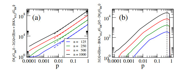
Figure 3.  Right hand side of (a) Eq (3.9) and (b) Eq (3.10) as a function of the probability $p$ of Erdős-Rényi graphs $G_{\mbox{ER}}(n, p)$ of size $n$. Each data value was computed by averaging over $10^{6}$ random graphs $G_{\mbox{ER}}(n, p)$. Dashed lines in (a) are Eq (3.11) with $\langle d_G \rangle = (n-1)p$. The dashed vertical line in (b) marks the maximum of the curves which occur at $p\approx 0.5$.

DownLoad: Full-Size Img PowerPoint

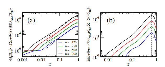
Figure 4.  Right hand side of (a) Eq (3.9) and (b) Eq (3.10) as a function of the connection radius $r$ of random geometric graphs $G_{\mbox{RG}}(n, r)$ of size $n$. Each data value was computed by averaging over $10^{6}$ random graphs $G_{\mbox{RG}}(n, r)$. Dashed lines in (a) are Eq (3.11) with $\langle d_G \rangle = (n-1)r^2(\pi-8r/3+r^2/2)$. The dashed vertical line in (b) marks the maximum of the curves which occur at $r\approx 0.64$.

DownLoad: Full-Size Img PowerPoint

Also, from Figure 3(a) [from Figure 4(a)] we observe that the right hand side of Eq (3.9) is close to zero for $n\to 0$ and $p\to 0$ [$r\to 0$], then grows with $p$ [$r$] approaching their maximum value at $p = 1$ [$r = \sqrt{2}$]. While from Figure 3(b) [from Figure 4(b)] we note that the right hand side of Eq (3.10) is close to zero for $n\to 0$ and $p\to 0$ [$r\to 0$], then grows with $p$ [$r$], approaches a maximum value at $p\approx 0.5$ [$r\approx 0.64$], and finally decrease abruptly and become zero at $p = 1$ [$r = \sqrt{2}$].

By the use of the same approximations that allowed us to get Eqs (3.7) and (3.8) in the previous subsection, we can also estimate the right hand side of Eq (3.9) for both ER and RG graphs in the dilute limit. This results in

Therefore, in Figure 3(a) [from Figure 4(a)] we plot Eq (3.11), as dashed lines, and observe good correspondence with the computational data.

4.   Conclusions

In this work, we study the recently introduced Revan Sombor index and the first and second Revan $(a, b)$-$KA$ indices. First, we present new relations to provide bounds on these Revan indices of the Sombor family which also serve to relate them with other Revan indices (such as $R_{1, 2}$, which are Revan versions of the first and second Zagreb indices) and with standard degree-based indices (such as the Sombor index, the first and second $(a, b)$-$KA$ indices, the first Zagreb index and the Harmonic index). We also quantify our relations on two models of random graphs: Erdös-Rényi graphs and random geometric graphs. Then, motivated by the growing interest in the application of topological indices in the analysis of random graphs, we extend some of our relations to index average values, so they can be effectively used for the statistical study of ensembles of random graphs. It is important to stress that our results on index average values are essentially obtained by averaging over the graph ensemble in the statistical sense rather than in the rigorous probabilistic sense, which is a topic we plan to explore in the near future.

We hope our results may motivate further analytical as well as computational studies of Revan Sombor indices. Indeed, since the average Sombor indices have shown to work as complexity measures of random graphs and networks (equivalent to random matrix theory measures) ^[32], we plan to explore wether Revan Sombor indices could also be used in this direction.

Acknowledgments

J. A. M. -B. thanks support from CONACyT (Grant No. 286633), CONACyT-Fronteras (Grant No. 425854), and VIEP-BUAP (Grant No. 100405811-VIEP2022), Mexico. The research of J. M. R. and J. M. S. was supported by a grant from Agencia Estatal de Investigación (PID2019-106433GBI00/AEI/10.13039/501100011033), Spain. J. M. R. was supported by the Madrid Government (Comunidad de Madrid-Spain) under the Multiannual Agreement with UC3M in the line of Excellence of University Professors (EPUC3M23), and in the context of the V PRICIT (Regional Programme of Research and Technological Innovation).

Conflict of interest

The authors declare there is no conflict of interest.