Loading [MathJax]/jax/output/SVG/jax.js
Research article Special Issues

Seasonal shifting of surplus renewable energy in a power system located in a cold region

  • The Fukushima nuclear disaster in 2011 changed Japan's strategy for reducing CO2 emissions. The government is now placing more emphasis on the development of nonCO2-emitting distributed generation systems such as wind, solar, and tidal power to reduce greenhouse gas emissions and guarantee electricity supply in the case of a natural disaster. This paper proposes a strategy for the exploitation of wind, solar, and tidal resources in a cold region in Japan by utilizing surplus energy from the summer and spring during winter. It also aims to determine the most favorable energy mix of these renewable sources and storage system types. The study is performed by calculating hourly demand and renewable energy supply for the city in one year, which is based on actual data of demand, solar irradiation, wind speeds, and tidal current speeds. The costs of the components of the renewable power plants and storage systems are considered, and different proportions of generation outputs are evaluated with different types of storage systems. According to results, the configuration containing the hydrogen storage system using organic chemical hydride methylcyclohexane (OCHM) is the most economical but is still more expensive than one using a conventional generation system. Moreover, we confirm that the cost of CO2 emissions is the key element for leveling the playing field between conventional and renewable generation from an economic perspective. The cost of CO2 emissions to public health as well as those costs related to the interruption of services during a catastrophe must be carefully calculated with other issues from conventional power projects to perform a precise comparative evaluation between both types of generation systems.

    Citation: Jorge Morel, Yuta Morizane, Shin'ya Obara. Seasonal shifting of surplus renewable energy in a power system located in a cold region[J]. AIMS Energy, 2014, 2(4): 373-384. doi: 10.3934/energy.2014.4.373

    Related Papers:

    [1] Wenjun Liu, Zhijing Chen, Zhiyu Tu . New general decay result for a fourth-order Moore-Gibson-Thompson equation with memory. Electronic Research Archive, 2020, 28(1): 433-457. doi: 10.3934/era.2020025
    [2] Siyi Luo, Yinghui Zhang . Space-time decay rate for the 3D compressible quantum magnetohydrodynamic model. Electronic Research Archive, 2025, 33(7): 4184-4204. doi: 10.3934/era.2025189
    [3] Yi Cheng, Ying Chu . A class of fourth-order hyperbolic equations with strongly damped and nonlinear logarithmic terms. Electronic Research Archive, 2021, 29(6): 3867-3887. doi: 10.3934/era.2021066
    [4] Mohammad M. Al-Gharabli, Adel M. Al-Mahdi . Existence and stability results of a plate equation with nonlinear damping and source term. Electronic Research Archive, 2022, 30(11): 4038-4065. doi: 10.3934/era.2022205
    [5] Chahrazed Messikh, Soraya Labidi, Ahmed Bchatnia, Foued Mtiri . Energy decay for a porous system with a fractional operator in the memory. Electronic Research Archive, 2025, 33(4): 2195-2215. doi: 10.3934/era.2025096
    [6] Jincheng Shi, Shuman Li, Cuntao Xiao, Yan Liu . Spatial behavior for the quasi-static heat conduction within the second gradient of type Ⅲ. Electronic Research Archive, 2024, 32(11): 6235-6257. doi: 10.3934/era.2024290
    [7] Jie Qi, Weike Wang . Global solutions to the Cauchy problem of BNSP equations in some classes of large data. Electronic Research Archive, 2024, 32(9): 5496-5541. doi: 10.3934/era.2024255
    [8] Xu Liu, Jun Zhou . Initial-boundary value problem for a fourth-order plate equation with Hardy-Hénon potential and polynomial nonlinearity. Electronic Research Archive, 2020, 28(2): 599-625. doi: 10.3934/era.2020032
    [9] Qin Ye . Space-time decay rate of high-order spatial derivative of solution for 3D compressible Euler equations with damping. Electronic Research Archive, 2023, 31(7): 3879-3894. doi: 10.3934/era.2023197
    [10] Huafei Di, Yadong Shang, Jiali Yu . Existence and uniform decay estimates for the fourth order wave equation with nonlinear boundary damping and interior source. Electronic Research Archive, 2020, 28(1): 221-261. doi: 10.3934/era.2020015
  • The Fukushima nuclear disaster in 2011 changed Japan's strategy for reducing CO2 emissions. The government is now placing more emphasis on the development of nonCO2-emitting distributed generation systems such as wind, solar, and tidal power to reduce greenhouse gas emissions and guarantee electricity supply in the case of a natural disaster. This paper proposes a strategy for the exploitation of wind, solar, and tidal resources in a cold region in Japan by utilizing surplus energy from the summer and spring during winter. It also aims to determine the most favorable energy mix of these renewable sources and storage system types. The study is performed by calculating hourly demand and renewable energy supply for the city in one year, which is based on actual data of demand, solar irradiation, wind speeds, and tidal current speeds. The costs of the components of the renewable power plants and storage systems are considered, and different proportions of generation outputs are evaluated with different types of storage systems. According to results, the configuration containing the hydrogen storage system using organic chemical hydride methylcyclohexane (OCHM) is the most economical but is still more expensive than one using a conventional generation system. Moreover, we confirm that the cost of CO2 emissions is the key element for leveling the playing field between conventional and renewable generation from an economic perspective. The cost of CO2 emissions to public health as well as those costs related to the interruption of services during a catastrophe must be carefully calculated with other issues from conventional power projects to perform a precise comparative evaluation between both types of generation systems.


    The Moore-Gibson-Thompson (MGT) equation is one of the equations of nonlinear acoustics describing acoustic wave propagation in gases and liquids [13,15,30] and arising from modeling high frequency ultrasound waves [9,18] accounting for viscosity and heat conductivity as well as effect of the radiation of heat on the propagation of sound. This research field is highly active due to a wide range of applications such as the medical and industrial use of high intensity ultrasound in lithotripsy, thermotherapy, ultraound cleaning, etc. The classical nonlinear acoustics models include the Kuznetson's equation, the Westervelt equation and the Kokhlov-Zabolotskaya-Kuznetsov equation.

    In order to gain a better understanding of the nonlinear MGT equation, we shall begin with the linearized model. In [15], Kaltenbacher, Lasiecka and Marchand investigated the following linearized MGT equation

    $ τuttt+αutt+c2Au+bAut=0. $ (1.1)

    For equation (1.1), they disclosed a critical parameter $ \gamma = \alpha-\frac{c^{2}\tau}{b} $ and showed that when $ \gamma>0 $, namely in the subcritical case, the problem is well-posed and its solution is exponentially stable; while $ \gamma = 0 $, the energy is conserved. Since its appearance, an increasing interest has been developed to study the MGT equation, see [4,5,8,10,14]. Caixeta, Lasiecka and Cavalcanti [4] considered the following nonlinear equation

    $ τuttt+αutt+c2Au+bAut=f(u,ut,utt). $ (1.2)

    They proved that the underlying PDE generates a well-posed dynamical system which admits a global and finite dimensional attractor. They also overcomed the difficulty of lacking the Lyapunov function and the lack of compactness of the trajectory.

    Now, we concentrate on the stabilization of MGT equation with memory which has received a considerable attention recently. For instance, Lasiecka and Wang [17] studied the following equation:

    $ τuttt+αutt+bAut+c2Aut0g(ts)Aw(s)ds=0, $ (1.3)

    where $ \alpha-\frac{c^{2}\tau}{b}\geq0 $ and the form of $ w $ classifies the memory into three types. By imposing the assumption on the relaxation function $ g $, for a positive constant $ c_{0} $, as

    $ g(t)c0g(t), $ (1.4)

    they discussed the effect of memory described by three types on decay rates of the energy when $ \alpha-\frac{c^{2}\tau}{b}>0 $. Moreover, in the critical case $ \alpha-\frac{c^{2}\tau}{b} = 0 $, they proved an exponential rate of decay for the solution of (1.3) under "the right mixture" of memory. Lasiecka and Wang [18] showed the general decay result of the equation (1.3) when $ w = u $, and established their result under weaker condition on $ g $. In [9], Filippo et al. investigated the critical case of equation (1.3) (that is $ \alpha b-c^{2}\tau = 0 $) for $ w = u $ and $ g $ satisfies (1.4), and obtained an exponential decay result if and only if $ \mathcal{A} $ is a bounded operator. When $ \int_{0}^{t} $ is replaced by $ \int_{0}^{\infty} $, (1.3) turns to

    $ τuttt+αutt+bAut+c2Au0g(s)Aw(ts)ds=0. $ (1.5)

    Alves et al. [1] investigated the uniform stability of equation (1.5) encompassing three different types of memory in a history space set by the linear semigroup theory. Moreover, we refer the reader to [3,6,7,12,24,25,26,28] for other works of the equation(s) with memory.

    More recently, Filippo and Vittorino [11] considered the fourth-order MGT equation

    $ utttt+αuttt+βutt+γAutt+δAut+ϱAu=0. $ (1.6)

    They investigated the stability properties of the related solution semigroup. And, according to the values of certain stability numbers depending on the strictly positive parameters $ \alpha $, $ \beta $, $ \gamma $, $ \delta $, $ \varrho $, they established the necessary and sufficient condition for exponential stability. For other related results on the higher-order equations, please see [20,27,34,35,36,37] and the references therein.

    Motivated by the above results, we intend to study the following abstract version of the fourth-order Moore-Gibson-Thompson (MGT) equation with a memory term

    $ utttt+αuttt+βutt+γAutt+δAut+ϱAut0g(ts)Au(s)ds=0, $ (1.7)

    where $ \alpha $, $ \beta $, $ \gamma $, $ \delta $, $ \varrho $ are strictly positive constants, $ \mathcal{A} $ is a strictly positive self-adjoint linear operator defined in a real Hilbert space $ H $ where the (dense) embedding $ \mathcal{D}(\mathcal{A})\subset H $ need not to be compact. And we consider the following initial conditions

    $ u(0)=u0,ut(0)=u1,utt(0)=u2,uttt(0)=u3. $ (1.8)

    A natural question that arised in dealing with the general decay of fourth-order MGT equation with memory:

    ● Can we get a general decay result for a class of relaxation functions satisfying $ g'(t)\leq-\xi(t)M(g(t)) $ for $ M $ to be increasing and convex function near the origin and $ \xi(t) $ to be a nonincreasing function?

    Mustafa answered this question for viscoelastic wave equations in [31,32]. Messaoudi and Hassan [29] considered the similar question for memory-type Timoshenko system in the cases of equal and non-equal speeds of wave propagation. Moreover, they extended the range of polynomial decay rate optimality from $ p\in\left[1,\frac{3}{2}\right) $ to $ p\in[1,2) $ when $ g $ satisfies $ g'(t)\leq-\xi(t)g^{p}(t) $. We refer to [19] for the non-equal wave speeds case. And, Liu et al. [22,23] also concerned with the similar question for third-order MGT equations with memory term.

    The aim of this paper is to establish the well-posedness and answer the above mention question for fourth-order MGT equation with memory (1.7). We first use the Faedo-Galerkin method to prove the well-posedness result. We then use the idea developed by Mustafa in [31,32], taking into consideration the nature of fourth-order MGT equation, to prove new general decay results for the case $ \gamma-\frac{\delta}{\alpha}>0 $ and $ \beta-\frac{\alpha\varrho}{\delta}>0 $, based on the perturbed energy method and on some properties of convex functions. Our result substantially improves and generalizes the earlier related results in previous literature.

    The rest of our paper is organized as follows. In Section $ 2 $, we give some assumptions and state our main results. In Section $ 3 $, we give the proof of well-posedness. In Section $ 4 $, we state and prove some technical lemmas that are relevant in the entire work. In Section $ 5 $, we prove the general decay result.

    In this section, we consider the following assumptions and state our main results. We use $ c>0 $ to denote a positive constant which does not depend on the initial data.

    First, we consider the following assumptions as in [11] for $ (A1) $, in [18] for $ (A3) $, $ (A5) $ and in [31] for $ (A2) $, $ (A4) $:

    $ {\rm (A1)} $ $ \gamma-\frac{\delta}{\alpha}>0 $ and $ \beta-\frac{\alpha\varrho}{\delta}>0 $.

    $ {\rm (A2)}\ g : \mathbb{R}^+\rightarrow\mathbb{R}^+\ $ is a non-increasing differentiable function such that

    $ 0 < g(0) < \frac{2\alpha\varrho}{\delta}(\alpha\gamma-\delta),\ \ \ \ \varrho-\int_{0}^{+\infty}g(s)ds = l > 0. $

    $ {\rm (A3)} $ $ g''(t)\geq 0 $ almost everywhere.

    $ {\rm (A4)} $ There exists a non-increasing differentiable function $ \xi $ : $ \mathbb{R}^+\rightarrow\mathbb{R}^+ $ and a $ C^{1} $ function $ M: $ $ [0,\infty)\rightarrow[0,\infty) $ which is either linear or strictly increasing and strictly convex $ C^{2} $ function on $ (0,r] $, $ r\leq g(0) $, with $ M(0) = M^{'}(0) = 0 $, such that

    $ g(t)ξ(t)M(g(t)), t0. $ (2.1)

    $ {\rm (A5)} $ There exists $ \lambda_{0}>0 $ such that $ \mathcal{A} $ satisfies $ \|u\|^{2}\leq \lambda_{0}\left\|\mathcal{A}^{\frac{1}{2}}u\right\|^{2} $ for all $ u\in H $.

    Remark 1. ([31,Remark 2.8]) (1) From assumption $ (A2) $, we deduce that

    $ g(t)0ast+andg(t)ϱlt, t>0. $

    Furthermore, from the assumption $ (A4) $, we obtain that there exists $ t_{0}\geq0 $ large enough such that

    $ g(t0)=randg(t)r, tt0. $

    The non-increasing property of $ g(t) $ and $ \xi(t) $ gives

    $ 0<g(t0)g(t)g(0)and0<ξ(t0)ξ(t)ξ(0), t[0,t0]. $

    A combination of these with the continuity of $ H $, for two constants $ a,d>0 $, yields

    $ aξ(t)M(g(t))d, t[0,t0]. $

    Consequently, for any $ t\in[0,t_{0}] $, we get

    $ g(t)ξ(t)M(g(t))a=ag(0)g(0)ag(0)g(t) $

    and, hence,

    $ g(t)g(0)ag(t), t[0,t0]. $ (2.2)

    (2) If $ M $ is a strictly increasing and strictly convex $ C^{2} $ function on $ (0,r] $, with $ M(0) = M'(0) = 0 $, then it has an extension $ \overline{M} $, which is strictly increasing and strictly convex $ C^{2} $ function on $ (0,\infty) $. For example, if we set $ M(r) = A $, $ M'(r) = B $, $ M''(r) = C $, we can define $ \overline{M} $, for any $ t>r $, by

    $ ¯M=C2t2+(BCr)t+(A+C2r2Br). $

    Then, inspired by the notations in [11], we define the Hilbert spaces

    $ Hr:=D(Ar2),rR. $

    In order to simplify the notation, we denote the usual space $ H_{0} $ by $ H $. The phase space of our problem is

    $ H=D(A12)×D(A12)×D(A12)×H. $

    Moreover, we will denote the inner product of $ H $ by $ (\cdot,\cdot) $ and its norm by $ \|\cdot\| $.

    After that, we introduce the following energy functional

    $ E(t)=12[uttt+αutt+αϱδut2+δα(ϱG(t)ϱ)A12utt+αA12ut+αϱδA12u2+δαϱG(t)A12utt+αA12ut2+(γδα)A12utt2+(γδα)αϱδA12ut2+2t0g(ts)(A12u(t)A12u(s),A12utt+αA12ut)ds+αϱδ(gA12u)(t)α(gA12u)(t)+αg(t)A12u2+(βαϱδ)utt2+αϱδ(βαϱδ)ut2], $

    where $ G(t) = \int_{0}^{t}g(s)ds $ and for any $ v\in L_{loc}^{2}\left(\mathbb{R}^{+};L^{2}(\Omega)\right) $,

    $ (gv)(t):=Ωt0g(ts)(v(t)v(s))2dsdx. $

    As in [31], we set, for any $ 0<\nu<1 $,

    $ Cν=0g2(s)νg(s)g(s)dsandh(t)=νg(t)g(t). $

    The following lemmas play an important role in the proof of our main results.

    Lemma 2.1. ([31] ) Assume that condition $ (A2) $ holds. Then for any $ u\in L_{loc}^{2}\left(\mathbb{R}^{+};\right. $ $ \left.L^{2}(\Omega)\right) $, we have

    $ Ω(t0g(ts)(A12u(s)A12u(t))ds)2dxCν(hA12u)(t), t0. $

    Lemma 2.2. (Jensen's inequality) Let $ P $: $ [b,c]\rightarrow \mathbb{R} $ be a convex function. Assume that functions $ f : \Omega\rightarrow [b,c] $ and $ h: \Omega\rightarrow \mathbb{R} $ are integrable such that $ h(x)\geq 0 $, for any $ x\in\Omega $ and $ \int_{\Omega} h(x)dx = k>0 $. Then

    $ P(1kΩf(x)h(x)dx)1kΩP(f(x))h(x)dx. $

    Lemma 2.3. ([2])(The generalized Young inequality) If $ f $ is a convex function defined on a real vector space $ X $ and ite convex conjugate is denoted by $ f^{*} $, then

    $ ABf(A)+f(B), $ (2.3)

    where

    $ f(s)=s(f)1(s)f[(f)1(s)]. $ (2.4)

    We are now in a position to state the well-posedness and the general decay result for problem (1.7)-(1.8).

    Theorem 2.4. (Well-posedness) Assume that $ (A1)-(A5) $ hold. Then, for given $ (u_{0}, u_{1}, u_{2}, u_{3})\in \mathcal{H} $ and $ T>0 $, there exists a unique weak solution $ u $ of problem (1.7)-(1.8) such that

    $ uC([0,T];D(A12))C1([0,T];H). $

    Theorem 2.5. (General decay) Let $ (u_{0},u_{1},u_{2},u_{3})\in\mathcal{H} $. Assume that $ (A1) $-$ (A5) $ hold. Then there exist positive constants $ k_{1} $ and $ k_{2} $ such that, along the solution of problem (1.7)-(1.8), the energy functional satisfies

    $ E(t)k2M11(k1tg1(r)ξ(s)ds), tg1(t), $ (2.5)

    where $ M_{1}(t) = \int_{t}^{r}\frac{1}{sM'(s)}ds $ and $ M_{1} $ is strictly decreasing and convex on $ (0,r] $, with $ {\lim\limits_{t\rightarrow 0}}M_{1}(t) = +\infty $.

    Remark 2. Assume that $ M(s) = s^{p} $, $ 1\leq p<2 $ in $ (A4) $, then by simple calculations, we see that the decay rate of $ E(t) $ is given by, for constants $ \overline{k} $, $ \widetilde{k} $ and $ C $,

    $ E(t){Cexp(˜kt0ξ(s)ds),ifp=1,¯k(1+t0ξ(s)ds)1p1,if1<p<2. $ (2.6)

    In this section, we will prove the global existence and uniqueness of the solution of problem (1.7)-(1.8). Firstly, we give the following lemmas.

    Lemma 3.1. If $ 0<g(0)<\frac{2\alpha\varrho}{\delta}(\alpha\gamma-\delta) $, then there is $ \sigma>0 $ such that $ \alpha\left(\gamma-\frac{\delta}{\alpha}\right)-\frac{\delta g(0)}{2(\alpha-\sigma)\varrho}>0 $.

    Proof. Since $ g(0)<\frac{2\alpha\varrho}{\delta}(\alpha\gamma-\delta) $, all we need is to show

    $ 2αϱδ(ασ)(γδα)2αϱδ(αγδ)asσ0, $

    which is trivially true.

    Lemma 3.2. Assume that $ (A1) $-$ (A5) $ hold. Then, the energy functional $ E(t) $ satisfies, for all $ t\geq 0 $,

    $ 12[uttt+αutt+αϱδut2+δα(ϱG(t)ϱ)A12utt+αA12ut+αϱδA12u2+(γδα)A12utt2+(γδα)αϱδA12ut2α(gA12u)(t)+αg(t)A12u2+(βαϱδ)utt2+αϱδ(βαϱδ)ut2]E(t)12[uttt+αutt+αϱδut2+δα(ϱG(t)ϱ)A12utt+αA12ut+αϱδA12u2+(γδα)A12utt2+(γδα)αϱδA12ut2α(gA12u)(t)+2αϱδ(gA12u)(t)+αg(t)A12u2+(βαϱδ)utt2+αϱδ(βαϱδ)ut2+2δαϱG(t)A12utt+αA12ut2]. $

    Proof. From the definition of $ E(t) $, we have

    $ E(t)=12[uttt+αutt+αϱδut2+δα(ϱG(t)ϱ)A12utt+αA12ut+αϱδA12u2+δαϱG(t)A12utt+αA12ut2+(γδα)A12utt2+(γδα)αϱδA12ut2+2t0g(ts)(A12u(t)A12u(s),A12utt+αA12ut)ds+αϱδ(gA12u)(t)α(gA12u)(t)+αg(t)A12u2+(βαϱδ)utt2+αϱδ(βαϱδ)ut2]. $

    Then, we estimate the sixth term of the above equality

    $ 2|t0g(ts)(A12u(t)A12u(s),A12utt+αA12ut)ds|t0g(ts)[αϱδA12u(t)A12u(s)2+δαϱA12utt+αA12ut2]ds=αϱδ(gA12u)(t)+δαϱG(t)A12utt+αA12ut2. $

    A combination of the above results, we complete the proof of lemma.

    Now, we prove the well-posedness result of problem (1.7)-(1.8).

    Proof of Theorem 2.1. The proof is given by Faedo-Galerkin method and combines arguments from [16,39,38]. We present only the main steps.

    Step $ 1 $. Approximate problem

    We construct approximations of the solution $ u $ by the Faedo-Galerkin method as follows. For every $ m\geq 1 $, let $ W_{m} = {\rm span}\{w_{1},\cdots, w_{m}\} $ be a Hilbertian basis of the space $ H^{1}_{0}(\Omega) $. We choose four sequences $ (u_{0}^{m}) $, $ (u_{1}^{m}) $, $ (u_{2}^{m}) $ and $ (u_{3}^{m}) $ in $ W_{m} $ such that $ u_{0}^{m}\rightarrow u_{0} $ strongly in $ \mathcal{D}\left(\mathcal{A}^{\frac{1}{2}}\right) $, $ u_{1}^{m}\rightarrow u_{1} $ strongly in $ \mathcal{D}\left(\mathcal{A}^{\frac{1}{2}}\right) $, $ u_{2}^{m}\rightarrow u_{2} $ strongly in $ \mathcal{D}\left(\mathcal{A}^{\frac{1}{2}}\right) $ and $ u_{3}^{m}\rightarrow u_{3} $ strongly in $ H $. We define now the approximations:

    $ um(t)=mj=1amj(t)wj(x), $ (3.1)

    where $ u^{m}(t) $ are solutions to the finite dimensional Cauchy problem (written in normal form):

    $ Ωumtttt(t)wjdx+αΩumttt(t)wjdx+βΩumtt(t)wjdx+γΩA12umtt(t)A12wjdx+δΩA12umt(t)A12wjdx+ϱΩA12um(t)A12wjdxt0g(ts)ΩA12um(t)A12wjdxds=0 $ (3.2)

    with initial conditions

    $ (um(0),umt(0),umtt(0),umttt(0))=(um0,um1,um2,um3). $ (3.3)

    According to the standard theory of ordinary differential equation, the finite dimensional problem (3.2)-(3.3) has a local solution $ \left(u^{m}(t), u^{m}_{t}(t),u^{m}_{tt}(t),u^{m}_{ttt}(t)\right) $ in some interval $ [0,T_{m}) $ with $ 0<T_{m}\leq T $, for every $ m\in \mathbb{N} $. Next, we present some estimates that allow us to extend the local solutions to the interval $ [0,T] $, for any given $ T>0 $.

    Step $ 2 $. Weak solutions

    Multiplying equation (3.2) by $ a_{jttt}^{m}+\alpha a_{jtt}^{m}+\frac{\alpha\varrho}{\delta}a_{jt}^{m} $ and integrating over $ \Omega $, we have

    $ ddtEm(t)+α(βαϱδ)umtt2αg(t)2A12um2+δ2αϱg(t)A12umtt+αϱδA12um2+α2(gA12um)(t)=[α(γδα)δg(t)2αϱ]A12umtt2+t0g(ts)(A12um(t)A12um(s),A12umtt)ds+αϱ2δ(gA12um)(t), $

    where

    $ Em(t)=12[umttt+αumtt+αϱδumt2+δα(ϱG(t)ϱ)A12umtt+αA12umt+αϱδA12um2+δαϱG(t)A12umtt+αA12umt2+(γδα)A12umtt2+(γδα)αϱδA12umt2+2t0g(ts)(A12um(t)A12um(s),A12umtt+αA12umt)ds+αϱδ(gA12um)(t)α(gA12um)(t)+αg(t)A12um2+(βαϱδ)umtt2+αϱδ(βαϱδ)umt2]. $ (3.4)

    From assumptions $ (A1)-(A3) $ and Lemma 3.1, we get, for $ \varepsilon\in(0,\alpha) $,

    $ t0g(ts)(A12um(t)A12um(s),A12umtt)ds(αε)ϱ2δ(gA12um)(t)δ2(αε)ϱA12umtt2t0g(ts)ds=(αε)ϱ2δ(gA12um)(t)+δ(g(0)g(t))2(αε)ϱA12umtt2 $

    and so

    $ [α(γδα)δg(t)2αϱ]A12umtt2+t0g(ts)(A12um(t)A12um(s),A12umtt)ds+αϱ2δ(gA12um)(t)[α(γδα)δg(t)2αϱ]A12umtt2(αε)ϱ2δ(gA12um)(t)+δ(g(0)g(t))2(αε)ϱA12umtt2+αϱ2δ(gA12um)(t)=[α(γδα)δg(0)2(αε)ϱ]A12umtt2+εϱ2δ(gA12um)(t)[δg(t)2(αε)ϱδg(t)2αϱ]A12umtt20. $ (3.5)

    Therefore, we have

    $ ddtEm(t)+α(βαϱδ)umtt2αg(t)2A12um2+δ2αϱg(t)A12umtt+αϱδA12um2+α2(gA12um)(t)0. $ (3.6)

    Integrating (3.6) from $ 0 $ to $ t\leq T_{m} $, one has

    $ Em(t)+t0[α(βαϱδ)umtt2αg(τ)2A12um2+δ2αϱg(τ)A12umtt+αϱδA12um2+α2(gA12um)(τ)]dτEm(0). $ (3.7)

    Now, since the sequences $ (u_{0}^{m})_{m\in N} $, $ (u_{1}^{m})_{m\in N} $, $ (u_{2}^{m})_{m\in N} $ and $ (u_{3}^{m})_{m\in N} $ converge and using $ (A1)-(A3) $, we can find a positive constant $ C $ independent of $ m $ such that

    $ Em(t)C. $ (3.8)

    Therefore, using the fact $ \varrho-\int_{0}^{t}g(s)ds\geq l $, the last estimate (3.8) together with (3.4) give us, for all $ m\in N, T_{m} = T $, we deduce that

    $ (um)mNisboundedinL(0,T;D(A12))(umt)mNisboundedinL(0,T;D(A12))(umtt)mNisboundedinL(0,T;D(A12))(umttt)mNisboundedinL(0,T;H). $ (3.9)

    Consequently, we may conclude that

    $ umuweakinL(0,T;D(A12))umtutweakinL(0,T;D(A12))umttuttweakinL(0,T;D(A12))umtttutttweakinL(0,T;H). $

    From (3.9), we get that $ (u^{m})_{m\in N} $ is bounded in $ L^{\infty}\left(0,T; \mathcal{D}\left(\mathcal{A}^{\frac{1}{2}}\right)\right) $. Then, $ (u^{m})_{m\in N} $ is bounded in $ L^{2}\left(0,T; \mathcal{D}\left(\mathcal{A}^{\frac{1}{2}}\right)\right) $. Since $ (u_{t}^{m})_{m\in N} $ is bounded in $ L^{\infty}\left(0,T; \mathcal{D}\left(\mathcal{A}^{\frac{1}{2}}\right)\right) $, $ (u_{t}^{m})_{m\in N} $ is bounded in $ L^{2}\left(0,T; \mathcal{D}\left(\mathcal{A}^{\frac{1}{2}}\right)\right) $. Consequently, $ (u_{tt}^{m})_{m\in N} $ is bounded in $ L^{2}\left(0,T; \mathcal{D}\left(\mathcal{A}^{\frac{1}{2}}\right)\right) $ and $ (u_{ttt}^{m})_{m\in N} $ is bounded in $ L^{2}\left(0,T; H\right) $. Moreover, $ (u^{m})_{m\in N} $ is bounded in $ H^{3}(0,T; H^{1}(\Omega)) $.

    Since the embedding $ H^{3}(0,T; H^{1}(\Omega))\hookrightarrow L^{2}(0,T; H(\Omega)) $ is compact, using Aubin-Lions theorem [21], we can extract a subsequence $ (u^{n})_{n\in N} $ of $ (u^{m})_{m\in N} $ such that

    $ unustronglyinL2(0,T;H(Ω)). $

    Therefore,

    $ unustronglyanda.e.on(0,T)×Ω. $

    The proof now can be completed arguing as in [21].

    Step $ 3 $. Uniqueness

    It is sufficient to show that the only weak solution of (1.7)-(1.8) with $ u_{0} = u_{1} = u_{2} = u_{3} = 0 $ is

    $ u0. $ (3.10)

    According to the energy estimate (3.8) and noting that $ E(u(0)) = 0 $, we obtain

    $ E(u(t))=0,t[0,T]. $

    So, we have

    $ uttt+αutt+αϱδut2=A12utt+αA12ut+αϱδA12u2=A12utt2=A12ut2=A12u2=utt2=0,t[0,T]. $

    And this implies (3.10). Thus, we conclude that problem (1.7)-(1.8) has at most one solution.

    In this section, we state and prove some lemmas needed to establish our general decay result.

    Lemma 4.1. Let $ (u,u_{t},u_{tt}, u_{ttt}) $ be the solution of (1.7). Assume that $ (A1) $-$ (A3) $ hold. Then, we have

    $ ddtE(t)α(βαϱδ)utt2[α(γδα)δg(0)2(αε)ϱ]A12utt2+αg(t)2A12u2[δg(t)2(αε)ϱδg(t)2αϱ]A12utt2δ2αϱg(t)A12utt+αϱδA12u2α2(gA12u)(t)+εϱ2δ(gA12u)0. $

    Proof. Multiplying (1.7) by $ u_{ttt}+\alpha u_{tt}+\frac{\alpha\varrho}{\delta}u_{t} $ and integrating over $ \Omega $ yield

    $ ddtE(t)=α(βαϱδ)utt2[α(γδα)δg(t)2αϱ]A12utt2+αg(t)2A12u2δ2αϱg(t)A12utt+αϱδA12u2+t0g(ts)(A12u(t)A12u(s),A12utt)dsα2(gA12u)(t)+αϱ2δ(gA12u)(t). $ (4.1)

    We proceed to show that, for a constant $ \varepsilon\in(0,\alpha) $,

    $ |t0g(ts)(A12u(t)A12u(s),A12utt)ds|(αε)ϱ2δ(gA12u)(t)+δ(g(0)g(t))2(αε)ϱA12utt2. $ (4.2)

    Then, combining (4.1) and (4.2), we can obtain

    $ ddtE(t)α(βαϱδ)utt2[α(γδα)δg(0)2(αε)ϱ]A12utt2+αg(t)2A12u2[δg(t)2(αε)ϱδg(t)2αϱ]A12utt2δ2αϱg(t)A12utt+αϱδA12u2α2(gA12u)(t)+εϱ2δ(gA12u). $

    According to $ (A1) $-$ (A3) $ and Lemma 3.1, we complete the proof of lemma.

    Lemma 4.2. Assume that $ (A1) $-$ (A5) $ hold. Then, the functional $ F_{1}(t) $ defined by

    $ F1(t)=Ω(utt+αut+αϱδu)(uttt+αutt+αϱδut)dx $

    satisfies the estimate

    $ F1(t)δ2αA12utt+αA12ut+αϱδA12u2+2αλ0δ(βαϱδ)2utt2+2αδ(γδα)2A12utt2+uttt+αutt+αϱδut2+2α(ϱl)2δA12u2+2αδCν(hA12u)(t). $ (4.3)

    Proof. Taking the derivative of $ F_{1}(t) $ with respect to $ t $, exploiting (1.7) and integrating by parts, we get

    $ F1(t)=Ω[(βαϱδ)utt](utt+αut+αϱδu)dxδαA12utt+αA12ut+αϱδA12u2+uttt+αutt+αϱδut2Ω(γδα)A12utt(A12utt+αA12ut+αϱδA12u)dx+Ω(t0g(ts)A12u(s)ds)(A12utt+αA12ut+αϱδA12u)dx. $

    Using Young's inequality, Lemma 2.1, $ (A5) $ and the fact $ \gamma-\frac{\delta}{\alpha}>0 $ and $ \beta-\frac{\alpha\varrho}{\delta}>0 $, we have

    $ Ω[(βαϱδ)utt](utt+αut+αϱδu)dx2αλ0δ(βαϱδ)2utt2+δ8αλ0utt+αut+αϱδu22αλ0δ(βαϱδ)2utt2+δ8αA12utt+αA12ut+αϱδA12u2 $

    and

    $ Ω(t0g(ts)A12u(s)ds)(A12utt+αA12ut+αϱδA12u)dx=Ω(t0g(ts)(A12u(s)A12u(t))ds)(A12utt+αA12ut+αϱδA12u)dx+Ω(t0g(ts)A12u(t)ds)(A12utt+αA12ut+αϱδA12u)dx2αδCν(hA12u)(t)+δ4αA12utt+αA12ut+αϱδA12u2+2α(ϱl)2δA12u2. $

    Also, we have

    $ Ω(γδα)A12utt(A12utt+αA12ut+αϱδA12u)dx2αδ(γδα)2A12utt2+δ8αA12utt+αA12ut+αϱδA12u2. $

    Then, combining the above inequalities, we complete the proof of (4.3).

    Lemma 4.3. Assume that $ (A1) $-$ (A5) $ hold. Then the functional $ F_{2}(t) $ defined by

    $ F2(t)=Ω(uttt+αutt+αϱδut)t0g(ts)[(utt+αut+αϱδu)(t)αϱδu(s)]dsdx $

    satisfies the estimate

    $ F2(t)G(t)4uttt+αutt+αϱδut2+[(ϱl)2α22ε1+4λ0g2(0)α2G(t)]A12ut2+[λ0(ϱl)22+(δ2α2+ϱ2)+3(ϱl)2]ε1A12utt+αA12ut+αϱδA12u2+[α2ϱ2(ϱl)2λ0ε12δ2+(ϱl)22ε1+3(ϱl)2(αϱδ)2ε1+(ϱl)22(αϱδ)2]A12u2+[(ϱl)22ε1+12ε1(γδα)2+12(αϱδ)2(γδα)2]A12utt2+[(ε1α2ϱ2λ04δ2+34ε1+1+αϱδ+2α4ϱ2λ0G(t)δ2)Cν+2α2ϱ2λ0G(t)δ2](hA12u)(t)+[2(βαϱδ)2ε1+4g2(0)G(t)]utt2, $ (4.4)

    where $ 0<\varepsilon_{1}<1 $.

    Proof. By differentiating $ F_{2}(t) $ with respect to $ t $, using (1.7) and integrating by parts, we obtain

    $ F2(t)=Ω[βutt+γAutt+δAut+ϱAut0g(ts)Au(s)dsαϱδutt]×t0g(ts)[(utt+αut+αϱδu)(t)αϱδu(s)]dsdxg(0)Ω(uttt+αutt+αϱδut)(utt+αut)dxΩ(uttt+αutt+αϱδut)t0g(ts)[(utt+αut+αϱδu)(t)αϱδu(s)]dsdxt0g(s)dsuttt+αutt+αϱδut2=Ω[(βαϱδ)utt+δα(Autt+αAut+αϱδAu)+(γδα)Auttt0g(s)dsAu(t)]t0g(ts)[(utt+αut+αϱδu)(t)αϱδu(s)]dsdxt0g(s)dsuttt+αutt+αϱδut2Ω(uttt+αutt+αϱδut)t0g(ts)[(utt+αut+αϱδu)(t)αϱδu(s)]dsdx+(t0g(s)ds)Ωt0g(ts)(Au(t)Au(s))ds(utt+αut)dx+αϱδΩ(t0g(ts)(A12u(t)A12u(s))ds)2dxg(0)Ω(uttt+αutt+αϱδut)(utt+αut)dx. $

    Now, we estimate the terms in the right-hand side of the above identity.

    Using Young's inequality, we obtain, for $ 0<\varepsilon_{1}<1 $,

    $ Ω[(βαϱδ)utt+δα(Autt+αAut+αϱδAu)+(γδα)Auttt0g(s)dsAu(t)]t0g(ts)[(utt+αut+αϱδu)αϱδu(s)]dsdx[λ0(ϱl)22+(δ2α2+ϱ2)+2(ϱl)2]ε1A12utt+αA12ut+αϱδA12u2+2(βαϱδ)2ε1utt2+[α2ϱ2(ϱl)2λ0ε12δ2+(ϱl)22ε1+2(ϱl)2(αϱδ)2ε1+(ϱl)22(αϱδ)2]A12u2+[(ϱl)22ε1+12ε1(γδα)2+12(αϱδ)2(γδα)2]A12utt2+(ϱl)2α22ε1A12ut2+(ε1α2ϱ2λ04δ2+14ε1+1)Cν(hA12u)(t) $

    and

    $ (t0g(s)ds)Ωt0g(ts)(Au(t)Au(s))ds(utt+αut)dx=(t0g(s)ds)Ωt0g(ts)(A12u(t)A12u(s))ds(A12utt+αA12ut)dx12ε1Cν(hA12u)(t)+(ϱl)22ε1A12utt+αA12ut212ε1Cν(hA12u)(t)+(ϱl)2ε1A12utt+αA12ut+αϱδA12u2+(ϱl)2(αϱδ)2ε1A12u2. $

    Also, we have

    $ αϱδΩ(t0g(ts)(A12u(t)A12u(s))ds)2dxαϱδCν(hA12u)(t) $

    and

    $ g(0)Ω(uttt+αutt+αϱδut)(utt+αut)dxG(t)4uttt+αutt+αϱδut2+g2(0)G(t)utt+αut2G(t)4uttt+αutt+αϱδut2+2g2(0)G(t)utt2+2λ0g2(0)α2G(t)A12ut2. $

    Exploiting Young's inequality and $ (A5) $, we get

    $ Ω(uttt+αutt+αϱδut)t0g(ts)[(utt+αut+αϱδu)(t)αϱδu(s)]dsdx=Ω(uttt+αutt+αϱδut)t0g(ts)(utt+αut)(t)dsdxαϱδΩ(uttt+αutt+αϱδut)t0g(ts)(u(t)u(s))dsdxG(t)2uttt+αutt+αϱδut2+2g2(0)G(t)utt2+2λ0α2g2(0)G(t)A12ut2+2α2ϱ2λ0G(t)δ2(α2Cν+1)(hA12u)(t). $

    A combination of all the above estimates gives the desired result.

    As in [11], we introduce the following auxiliary functional

    $ F3(t)=Ω(uttt+αutt)utdx+ϱ2A12u2. $

    Lemma 4.4. Assume that $ (A1) $-$ (A5) $ hold. Then the functional $ F_{3}(t) $ satisfies the estimate

    $ F3(t)(3δ8ε2δ4)A12ut2+ε2δ38α2ϱ2λ0uttt+αutt+αϱδut2+2γ2δA12utt2+(ε2δ34ϱ2λ0+4α2ϱ2λ0ε2δ3+2β2λ0δ)utt2+1δCν(hA12u)(t)+2(ϱl)2δA12u2, $ (4.5)

    where $ 0<\varepsilon_{2}<1 $.

    Proof. Using the equation (1.7), a direct computation leads to the following identity

    $ F3(t)=Ω(uttt+αutt)uttdx+Ω(utttt+αuttt)utdx+ϱ(A12u,A12ut)=(uttt,utt)+αutt2β(utt,ut)γ(A12utt,A12ut)δA12ut2+(t0g(ts)A12u(s)ds,A12ut). $ (4.6)

    Now, the first and third terms in the right-hand side of (4.6) can be estimated as follows:

    $ (uttt,utt)ε2δ316α2ϱ2λ0uttt2+4α2ϱ2λ0ε2δ3utt2ε2δ38α2ϱ2λ0uttt+αutt+αϱδut2+ε2δ38α2ϱ2λ0αutt+αϱδut2+4α2ϱ2λ0ε2δ3utt2ε2δ38α2ϱ2λ0uttt+αutt+αϱδut2+α2(ε2δ34α2ϱ2λ0+4ϱ2λ0ε2δ3)utt2+ε2δ4A12ut2 $

    and

    $ β(utt,ut)2β2λ0δutt2+δ8λ0ut22β2λ0δutt2+δ8A12ut2, $

    where $ 0<\varepsilon_{2}<1 $.

    Using Young's inequality and Lemma 2.1, we get

    $ γ(A12utt,A12ut)2γ2δA12utt2+δ8A12ut2 $

    and

    $ (t0g(ts)A12u(s)ds,A12ut)=(t0g(ts)(A12u(s)A12u(t)+A12u(t))ds,A12ut)1δΩ(t0g(ts)(A12u(t)A12u(s))ds)2dx+δ4A12ut2+2(ϱl)2δA12u2+δ8A12ut21δCν(hA12u)(t)+3δ8A12ut2+2(ϱl)2δA12u2. $

    Then, combining the above inequalities, we obtain the desired result.

    Lemma 4.5. Assume that $ (A1) $-$ (A5) $ hold. Then the functional $ F_{4}(t) $ defined by

    $ F4(t)=Ωt0f(ts)|A12u(s)|2dsdx $

    satisfies the estimate

    $ F4(t)12(gA12u)(t)+3(ϱl)A12u2, $ (4.7)

    where $ f(t) = \int_{t}^{\infty}g(s)ds $.

    Proof. Noting that $ f'(t) = -g(t) $, we see that

    $ F4(t)=f(0)A12u2Ωt0g(ts)|A12u(s)|2dsdx=f(0)A12u2Ωt0g(ts)|A12u(s)A12u(t)|2dsdx2ΩA12ut0g(ts)(A12u(s)A12u(t))dsdx(t0g(s)ds)A12u2=(gA12u)(t)2ΩA12ut0g(ts)(A12u(s)A12u(t))dsdx+f(t)A12u2. $

    Exploiting Young's inequality and the fact $ \int_{0}^{t}g(s)ds\leq \varrho-l $, we obtain

    $ 2ΩA12ut0g(ts)(A12u(s)A12u(t))dsdx2(ϱl)A12u2+12(ϱl)(t0g(ts)ds)Ωt0g(ts)(A12u(s)A12u(t))2dsdx2(ϱl)A12u2+12(gA12u)(t). $

    Moreover, taking account of $ f(t)\leq f(0) = \varrho-l $, we have

    $ f(t)A12u2(ϱl)A12u2. $

    Combining the above estimates, we arrive at the desired result.

    Lemma 4.6. Assume that $ (A1)-(A5) $ hold. The functional $ \mathcal{L}(t) $ defined by

    $ L(t)=NE(t)+F1(t)+N2F2(t)+N3F3(t) $

    satisfies, for a suitable choice of $ N, N_{2}, N_{3} $,

    $ L(t)E(t) $

    and the estimate, for all $ t\geq t_{0} $,

    $ L(t)c[utt2+A12utt2+uttt+αutt+αϱδut2+A12utt+αA12ut+αϱδu2]4(ϱl)A12u2+18(gA12u)(t), $ (4.8)

    where $ t_{0} $ has been introduced in Remark $ 2.1 $.

    Proof. Combining Lemmas 4.1-4.4 and recalling that $ g' = \nu g-h $, we obtain, for all $ t\geq t_{0} $,

    $ L(t)[α(βαϱδ)N2αλ0δ(βαϱδ)2(2(βαϱδ)2ε1+4g2(0)G(t))N2(ε2δ34ϱ2λ0+4α2ϱ2λ0ε2δ3+2β2λ0δ)N3]utt2[(α(γδα)δg(0)2(αε)ϱ)N+(δg(t)2(αε)ϱδg(t)2αϱ)N2αδ(γδα)2((ϱl)22ε1+12ε1(γδα)2+12(αϱδ)2(γδα)2)N22γ2δN3]A12utt2α2N(gA12u)(t)[(3δ8ε2δ4)N3((ϱl)2α22ε1+4λ0g2(0)α2G(t))N2]A12ut2(G(t)4N21ε2δ3N38α2ϱ2λ0)uttt+αutt+αϱδut2+εϱν2δN(gA12u)(t)[δ2α(λ0(ϱl)22+(δ2α2+ϱ2)+3(ϱl)2)ε1N2]×A12utt+αA12ut+αϱδA12u2[αg(t)2N2α(ϱl)2δ(α2ϱ2(ϱl)2λ0ε12δ2+(ϱl)22ε1+3(ϱl)2(αϱδ)2ε1+(ϱl)22(αϱδ)2)N22(ϱl)2δN3]A12u2[εϱ2δN2αδCν((ε1α2ϱ2λ04δ2+34ε1+1+αϱδ+2α4ϱ2λ0G(t)δ2)Cν+2α2ϱ2λ0G(t)δ2)N2N3δCν](hA12u)(t). $

    At this point, we need to choose our constants very carefully. First, we choose

    $ ε1=αδ2N2[λ0α2(ϱl)2+2(δ2+α2ϱ2)+6α2(ϱl)2]andε2=1N3. $

    The above choice yields

    $ L(t)[α(βαϱδ)N2αλ0δ(βαϱδ)2(2(βαϱδ)2ε1+4g2(0)G(t))N2δ34ϱ2λ04α2ϱ2λ0δ3N232β2λ0δN3]utt2[(α(γδα)δg(0)2(αε)ϱ)N+(δg(t)2(αε)ϱδg(t)2αϱ)N2αδ(γδα)2((ϱl)22ε1+12ε1(γδα)2+12(αϱδ)2(γδα)2)N22γ2δN3]A12utt2α2N(gA12u)(t)[3δ8N3δ4((ϱl)2α22ε1+4λ0g2(0)α2G(t))N2]A12ut2+εϱν2δN(gA12u)(t)(G(t)4N21δ38α2ϱ2λ0)uttt+αutt+αϱδut2δ4αA12utt+αA12ut+αϱδA12u2[αg(t)2N2α(ϱl)2δ(α2ϱ2(ϱl)2λ0ε12δ2+(ϱl)22ε1+3(ϱl)2(αϱδ)2ε1+(ϱl)22(αϱδ)2)N22(ϱl)2δN3]A12u2[εϱ2δN2αδCν((ε1α2ϱ2λ04δ2+34ε1+1+αϱδ+2α4ϱ2λ0G(t)δ2)Cν+2α2ϱ2λ0G(t)δ2)N2N3δCν](hA12u)(t). $

    Then, we choose $ N_{2} $ large enough so that

    $ G(t)4N21δ38α2ϱ2λ0>0. $

    Next, we choose $ N_{3} $ large enough so that

    $ 3δ8N3δ4((ϱl)2α22ε1+4λ0g2(0)α2G(t))N2>0. $

    Now, as $ \frac{\nu^{2}g(s)}{\nu g(s)-g'(s)}<g(s) $, it is easy to show, using the Lebesgue dominated convergence theorem, that

    $ νCν=0ν2g(s)νg(s)g(s)ds0,asν0. $

    Hence, there is $ 0<\nu_{0}<1 $ such that if $ \nu<\nu_{0} $, then

    $ νCν<116(2αδ+(ε1α2ϱ2λ04δ2+34ε1+1+αϱδ+2α4ϱ2λ0G(t)δ2)N2+N3δ). $

    Now, let us choose $ N $ large enough and choose $ \nu $ satisfying

    $ εϱ4δN2α2ϱ2λ0G(t)δ2N2>0andν=δ4εϱN<ν0, $

    which means

    $ εϱ2δN2α2ϱ2λ0G(t)δ2N2Cν(2αδ+(ε1α2ϱ2λ04δ2+34ε1+1+αϱδ+2α4ϱ2λ0G(t)δ2)N2+N3δ)>εϱ2δN2α2ϱ2λ0G(t)δ2N2116ν=εϱ4δN2α2ϱ2λ0G(t)δ2N2>0 $

    and

    $ α(βαϱδ)N2αλ0δ(βαϱδ)2(2(βαϱδ)2ε1+4g2(0)G(t))N2δ34ϱ2λ04α2ϱ2λ0δ3N232β2λ0δN3>0,(α(γδα)δg(0)2(αε)ϱ)N+(δg(t)2(αε)ϱδg(t)2αϱ)N2αδ(γδα)2((ϱl)22ε1+12ε1(γδα)2+12(αϱδ)2(γδα)2)N22γ2δN3>0,αg(t)2N2α(ϱl)2δ(α2ϱ2(ϱl)2λ0ε12δ2+(ϱl)22ε1+3(ϱl)2(αϱδ)2ε1+(ϱl)22(αϱδ)2)N22(ϱl)2δN3>4(ϱl). $

    So we arrive at, for positive constant $ c $,

    $ L(t)c[utt2+A12utt2+uttt+αutt+αϱδut2+A12utt+αA12ut+αϱδu2]4(ϱl)A12u2+18(gA12u)(t). $

    On the other hand, from Lemma 3.2, we find that

    $ |L(t)NE(t)|Ω|utt+αut+αϱδu||uttt+αutt+αϱδut|dx+N2Ω|uttt+αutt+αϱδut|t0g(ts)×|(utt+αut+αϱδu)(t)αϱδu(s)|dsdx+N3Ω|uttt+αutt||ut|dx+N3ϱ2A12u2cE(t). $

    Therefore, we can choose $ N $ even large (if needed) so that (4.8) is satisfied.

    In this section, we will give an estimate to the decay rate for the problem (1.7)-(1.8).

    Proof of Theorem 2.2. Our proof starts with the observation that, for any $ t\geq t_{0} $,

    $ t00g(s)Ω|A12u(t)A12u(ts)|2dxdsg(0)at00g(s)Ω|A12u(t)A12u(ts)|2dxdsg(0)at0g(s)Ω|A12u(t)A12u(ts)|2dxdscE(t), $

    which are derived from (2.2) and Lemma 4.1 and can be used in (4.8).

    Taking $ \mathcal{F}(t) = \mathcal{L}(t)+cE(t) $, which is obviously equivalent to $ E(t) $, we get, for all $ t\geq t_{0} $,

    $ L(t)c[utt2+A12utt2+uttt+αutt+αϱδut2+A12utt+αA12ut+αϱδu2]4(ϱl)A12u2+18(gA12u)(t)mE(t)+c(gA12u)(t)mE(t)cE(t)+ctt0g(s)Ω|A12u(t)A12u(ts)|2dxds, $

    where $ m $ is a positive constant. Then, we obtain that

    $ F(t)=L(t)+cE(t)mE(t)+ctt0g(s)Ω|A12u(t)A12u(ts)|2dxds. $ (5.1)

    We consider the following two cases relying on the ideas presented in [31].

    (ⅰ) $ M(t) $ is linear.

    We multiply (5.1) by $ \xi(t) $, then on account of $ (A1) $-$ (A4) $ and Lemma 4.1, we obtain, for all $ t\geq t_{0} $,

    $ ξ(t)F(t)mξ(t)E(t)+cξ(t)tt0g(s)Ω|A12u(t)A12u(ts)|2dxdsmξ(t)E(t)+ctt0ξ(s)g(s)Ω|A12u(t)A12u(ts)|2dxdsmξ(t)E(t)ctt0g(s)Ω|A12u(t)A12u(ts)|2dxdsmξ(t)E(t)ct0g(s)Ω|A12u(t)A12u(ts)|2dxdsmξ(t)E(t)cE(t). $

    Therefore,

    $ ξ(t)F(t)+cE(t)mξ(t)E(t). $

    As $ \xi(t) $ is non-increasing and $ \mathcal{F}(t)\sim E(t) $, we have

    $ ξ(t)F(t)+cE(t)E(t) $

    and

    $ (ξF+cE)(t)mξ(t)E(t), tt0. $

    It follows immediately that

    $ E(t)mξ(t)E(t), tt0. $

    We may now integrate over $ (t_{0},t) $ to conclude that, for two positive constants $ k_{1} $ and $ k_{2} $

    $ E(t)k2exp(k1tt0ξ(s)ds), tt0. $

    By the continuity of $ E(t) $, we have

    $ E(t)k2exp(k1t0ξ(s)ds), t>0. $

    (ⅱ) $ M $ is nonlinear.

    First, we define the functional

    $ L(t)=L(t)+F4(t). $

    Obviously, $ L(t) $ is nonnegative. And, by Lemma 4.5 and Lemma 4.6, there exists $ b>0 $ such that

    $ L(t)=L(t)+F4(t)c[utt2+A12utt2+uttt+αutt+αϱδut2+A12utt+αA12ut+αϱδu2](ϱl)A12u238(gA12u)(t)bE(t). $

    Therefore, integrating the above inequality over $ (t_{0},t) $, we see at once that

    $ L(t0)L(t)L(t0)btt0E(s)ds. $

    It is sufficient to show that

    $ 0E(s)ds< $ (5.2)

    and

    $ E(t)ctt0,t>t0. $

    Now, we define a functional $ \lambda(t) $ by

    $ λ(t):=tt0g(s)A12u(t)A12u(ts)2ds. $

    Clearly, we have

    $ λ(t)t0g(s)A12u(t)A12u(ts)2dscE(t), tt0. $ (5.3)

    After that, we define another functional $ I(t) $ by

    $ I(t):=qtt0A12u(t)A12u(ts)2ds. $

    Now, the following inequality holds under Lemma 4.1 and (5.2) that

    $ tt0A12u(t)A12u(ts)2ds2tt0(A12u(t)2+A12u(ts)2)ds4tt0(E(t)+E(ts))ds8tt0E(0)ds<. $ (5.4)

    Then (5.4) allows for a constant $ 0<q<1 $ chosen so that, for all $ t\geq t_{0} $,

    $ 0<I(t)<1; $ (5.5)

    otherwise we get an exponential decay from (5.1). Moreover, recalling that $ M $ is strict convex on $ (0,r] $ and $ M(0) = 0 $, then

    $ M(θx)θM(x),for0θ1andx(0,r]. $

    From assumptions $ (A2) $ and $ (A4) $, (5.5) and Lemma 2.2, it follows that

    $ λ(t)=tt0g(s)A12u(t)A12u(ts)2ds=1qI(t)tt0I(t)(g(s))qA12u(t)A12u(ts)2ds1qI(t)tt0I(t)ξ(s)M(g(s))qA12u(t)A12u(ts)2dsξ(t)qI(t)tt0M(I(t)g(s))qA12u(t)A12u(ts)2dsξ(t)qM(1I(t)tt0I(t)g(s)qA12u(t)A12u(ts)2ds)=ξ(t)qM(qtt0g(s)A12u(t)A12u(ts)2ds). $

    According to $ \overline{M} $ is an extension of $ M $ (see Remark $ 2.1 (2) $), we also have

    $ λ(t)ξ(t)q¯M(qtt0g(s)A12u(t)A12u(ts)2ds). $

    In this way,

    $ tt0g(s)A12u(t)A12u(ts)2ds1q¯M1(qλ(t)ξ(t)) $

    and (5.1) becomes

    $ F(t)mE(t)+ctt0g(s)Ω|A12u(t)A12u(ts)|2dxdsmE(t)+c¯M1(qλ(t)ξ(t)), tt0. $ (5.6)

    Let $ 0<\varepsilon_{0}<r $, we define the functional $ \mathcal{F}_{1}(t) $ by

    $ F1(t):=¯M(ε0E(t)E(0))F(t)+E(t), t0. $

    Then, recalling that $ E'(t)\leq 0 $, $ \overline{M}'>0 $ and $ \overline{M}''>0 $ as well as making use of estimate (5.6), we deduce that $ \mathcal{F}_{1}(t)\sim E(t) $ and also, for any $ t\geq t_{0} $, we have

    $ F1(t)mE(t)¯M(ε0E(t)E(0))+c¯M(ε0E(t)E(0))¯M1(qλ(t)ξ(t))+E(t). $ (5.7)

    Taking account of Lemma 2.3, we obtain

    $ ¯M(ε0E(t)E(0))¯M1(qλ(t)ξ(t))¯M(¯H(ε0E(t)E(0)))+¯M(¯M1(qλ(t)ξ(t)))=¯M(¯M(ε0E(t)E(0)))+qλ(t)ξ(t) $ (5.8)

    where

    $ ¯M(¯M(ε0E(t)E(0)))=¯M(ε0E(t)E(0))(¯M)1(¯M(ε0E(t)E(0)))¯M[(¯M)1(¯M(ε0E(t)E(0)))]=ε0E(t)E(0)¯M(ε0E(t)E(0))¯M(ε0E(t)E(0))ε0E(t)E(0)¯M(ε0E(t)E(0)). $ (5.9)

    So, combining (5.7), (5.8) and (5.9), we obtain

    $ F1(t)(mE(0)cε0)E(t)E(0)¯M(ε0E(t)E(0))+cqλ(t)ξ(t)+E(t). $

    From this, we multiply the above inequality by $ \xi(t) $ to get

    $ ξ(t)F1(t)(mE(0)cε0)ξ(t)E(t)E(0)¯M(ε0E(t)E(0))+cqλ(t)+ξ(t)E(t). $

    Then, using the fact that, as $ \varepsilon_{0}\frac{E(t)}{E(0)}<r $, $ \overline{M}'\left(\varepsilon_{0}\frac{E(t)}{E(0)}\right) = M'\left(\varepsilon_{0}\frac{E(t)}{E(0)}\right) $ and (5.3), we get

    $ ξ(t)F1(t)(mE(0)cε0)ξ(t)E(t)E(0)M(ε0E(t)E(0))cE(t). $

    Consequently, defining $ \mathcal{F}_{2}(t) = \xi(t)\mathcal{F}_{1}(t)+cE(t) $, then since $ \mathcal{F}_{1}(t)\sim E(t) $, we arrive at

    $ F2(t)E(t), $ (5.10)

    and with a suitable choice of $ \varepsilon_{0} $, we get, for some positive constant $ k $ and for any $ t\geq t_{0} $,

    $ F2(t)kξ(t)(E(t)E(0))M(ε0E(t)E(0)). $ (5.11)

    Define

    $ R(t)=λ1F2(t)E(0),λ1>0andM2(t)=tM(ε0t). $

    Moreover, it suffices to show that $ M'_{2}(t), M_{2}(t)>0 $ on $ (0,1] $ by the strict convexity of $ M $ on $ (0,r] $. And, it is easily seen that

    $ F2(t)kξ(t)M2(E(t)E(0)). $ (5.12)

    According to (5.10) and (5.12), there exist $ \lambda_{2}, \lambda_{3}>0 $ such that

    $ λ2R(t)E(t)λ3R(t). $ (5.13)

    Then, it follows that there exists $ k_{1}>0 $ such that

    $ k1ξ(t)R(t)M2(R(t)), tt0. $ (5.14)

    Next, we define

    $ M1(t):=rt1sM(s)ds. $

    And based on the properties of $ M $, we know that $ M_{1} $ is strictly decreasing function on $ (0,r] $ and $ {\lim_{t\rightarrow 0}}M_{1}(t) = +\infty $.

    Now, we integrate (5.14) over $ (t_{0},t) $ to obtain

    $ tt0R(s)M2(R(s))dsk1tt0ξ(s)ds $

    so

    $ k1tt0ξ(s)dsM1(ε0R(t))M1(ε0R(t0)), $

    which implies that

    $ M1(ε0R(t))k1tt0ξ(s)ds. $

    It is easy to obtain that

    $ R(t)1ε0M11(k1tt0ξ(s)ds), tt0. $ (5.15)

    A combining of (5.13) and (5.15) gives the proof.

    The authors are grateful to the anonymous referees and the editor for their useful remarks and comments.

    [1] Ministry of Economy, Trade and Industry (METI), Annual Report on Energy, Outline of the FY2012 (Energy White Paper 2013). Ministry of Economy, Trade and Industry (METI), 2013. Available from: http://www.meti.go.jp/english/report/index_whitepaper.html#energy.
    [2] New Energy and Industrial Technology Development Organization (NEDO), Demonstration Research on Japan's First Offshore Wind Turbines. New Energy and Industrial Technology Development Organization (NEDO), 2013. Available from:http://www.nedo.go.jp/english/introducing_project_02.html.
    [3] Japan Smart Community Alliance, The Operational Experience of Sendai Microgrid in the Aftermath of the Devastating Earthquake: A Case Study. New Energy and Industrial Technology Development Organization (NEDO), 2013. Available from: https://www.smart-japan.org/english/reference/l3/Vcms3_00000020.html.
    [4] Ma C, Zhang X, Zhang G, et al. (2013) Global utilization of solar energy and development of solar cell materials. Adv Mater Res 608: 151-154.
    [5] Zhang X, Ma C, Chen W, et al. (2013) Global utilization and development of wind energy. Adv Mater Res 608: 584-587.
    [6] Obara S (2008) Development of a dynamic operational scheduling algorithm for an independent micro-grid with renewable energy. J Therm Sci Tech-Jpn 3: 474-485. doi: 10.1299/jtst.3.474
    [7] U.S. Department of Energy, Microgrids at Berkeley Laboratory, Nagoya 2007 Symposium on Microgrids, Overview of Micro-grid R&D in Japan. New Energy and Industrial Technology Development Organization (NEDO), 2007. Available from: http://der.lbl.gov/sites/der.lbl.gov/files/nagoya_morozumi.pdf.
    [8] Obara S, Morizane Y, Morel J (2013) Economic efficiency of a renewable energy independent microgrid with energy storage by a sodium-sulfur battery or organic chemical hydride. Int J Hydrogen Energ 38: 8888-8902. doi: 10.1016/j.ijhydene.2013.05.036
    [9] Obara S, Morel J (2014) Microgrid composed of three or more SOFC combined cycles without accumulation of electricity. Int J Hydrogen Energ 39: 2297-2312. doi: 10.1016/j.ijhydene.2013.11.102
    [10] Obara S, Kawae O, Morizane Y, et al. (2013) The facility planning and electric power quality of the Saroma Lake green microgrid by the interconnection of tidal power generation, PV and SOFC. J Power Energ Syst 7: 1-17. doi: 10.1299/jpes.7.1
    [11] Obara S, Kawae O, Kawai M, et al. (2013) A study of the installed capacity and electricity quality of a fuel cell-independent microgrid that uses locally produced energy for local consumption. Int J Energy Res 37: 1764-1783. doi: 10.1002/er.2990
    [12] Obara S, Kawai M, Kawae O, et al. (2013) Operational planning for an independent microgrid containing tidal power generators, SOFCs, and photovoltaics. Appl Energ 102: 1343-1357. doi: 10.1016/j.apenergy.2012.07.005
    [13] Japan Meteorological Agency. Available from: http://www.jma.go.jp/jma/indexe.html. (In Japanese)
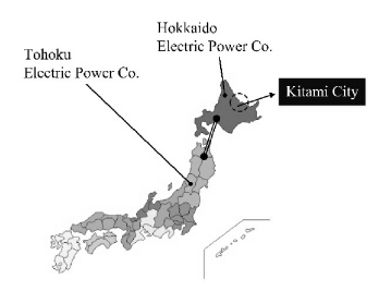
    [14] Hokkaido Electric Power Company, Main Infrastructure. Available from: http://www.hepco.co.jp/corporate/ele_power/ele_power.html. (In Japanese)
    [15] New Energy and Energy Saving Vision for Kitami City, 2012. (In Japanese)
    [16] Oxera Consulting Ltd., Discount rates for low-carbon and renewable generation technologies, 2011. Available from: http://www.oxera.com/Oxera/media/Oxera/downloads/reports/Oxera-report-on-low-carbon-discount-rates.pdf?ext=.pdf.
    [17] Trading Economics, Japan Inflation Rate 1958-2014, 2014. Available from: http://www.tradingeconomics.com/japan/inflation-cpi.
    [18] Ernst&Young, Black&Veath, Cost of and financial support for wave, tidal stream and tidal range generation in the UK, 2010. Available from: http://webarchive.nationalarchives.gov.uk/20121205174605/http:/decc.gov.uk/assets/decc/what%20we%20do/uk%20energy%20supply/energy%20mix/renewable%20energy/explained/wave_tidal/798-cost-of-and-finacial-support-for-wave-tidal-strea.pdf.
    [19] National Renewable Energy Laboratory (NREL), Distributed Generation Renewable Energy Estimate of Costs, 2013. Available from: http://www.nrel.gov/analysis/tech_lcoe_re_cost_est.html.The Economists, Companies and Emissions — Carbon Copy, 2013.
    [20] Available from: http://www.economist.com/news/business/21591601-some-firms-are-preparing-carbon-price-would-make-big-difference-carbon-copy.
  • This article has been cited by:

    1. Zhiyu Tu, Wenjun Liu, Well‐posedness and exponential decay for the Moore–Gibson–Thompson equation with time‐dependent memory kernel, 2023, 0170-4214, 10.1002/mma.9133
    2. Marina Murillo‐Arcila, Well‐posedness for the fourth‐order Moore–Gibson–Thompson equation in the class of Banach‐space‐valued Hölder‐continuous functions, 2023, 46, 0170-4214, 1928, 10.1002/mma.8618
    3. Carlos Lizama, Marina Murillo-Arcila, Well-posedness for a fourth-order equation of Moore–Gibson–Thompson type, 2021, 14173875, 1, 10.14232/ejqtde.2021.1.81
    4. Danhua Wang, Wenjun Liu, Well-posedness and decay property of regularity-loss type for the Cauchy problem of the standard linear solid model with Gurtin–Pipkin thermal law, 2021, 123, 18758576, 181, 10.3233/ASY-201631
    5. Yang Liu, Wenke Li, A class of fourth-order nonlinear parabolic equations modeling the epitaxial growth of thin films, 2021, 14, 1937-1632, 4367, 10.3934/dcdss.2021112
    6. Danhua Wang, Wenjun Liu, Kewang Chen, Well-posedness and decay property for the Cauchy problem of the standard linear solid model with thermoelasticity of type III, 2023, 74, 0044-2275, 10.1007/s00033-023-01964-4
    7. Doaa Atta, Ahmed E. Abouelregal, Hamid M. Sedighi, Rasmiyah A. Alharb, Thermodiffusion interactions in a homogeneous spherical shell based on the modified Moore–Gibson–Thompson theory with two time delays, 2023, 1385-2000, 10.1007/s11043-023-09598-9
    8. İbrahim TEKİN, Identification of the time-dependent lowest term in a fourth order in time partial differential equation, 2023, 72, 1303-5991, 500, 10.31801/cfsuasmas.1127250
    9. Husam Alfadil, Ahmed E. Abouelregal, Marin Marin, Erasmo Carrera, Goufo-Caputo fractional viscoelastic photothermal model of an unbounded semiconductor material with a cylindrical cavity, 2023, 1537-6494, 1, 10.1080/15376494.2023.2278181
    10. Danhua Wang, Wenjun Liu, Global Existence and Decay Property for the Cauchy Problem of the Nonlinear MGT Plate Equation, 2024, 89, 0095-4616, 10.1007/s00245-024-10126-5
    11. Flank D. M. Bezerra, Lucas A. Santos, Maria J. M. Silva, Carlos R. Takaessu, A Note on the Spectral Analysis of Some Fourth-Order Differential Equations with a Semigroup Approach, 2023, 78, 1422-6383, 10.1007/s00025-023-01999-z
    12. Carlos Lizama, Marina Murillo-Arcila, On the existence of chaos for the fourth-order Moore–Gibson–Thompson equation, 2023, 176, 09600779, 114123, 10.1016/j.chaos.2023.114123
    13. Wen-jun Liu, Zhi-yu Tu, Equivalence between the internal observability and exponential decay for the Moore-Gibson-Thompson equation, 2024, 39, 1005-1031, 89, 10.1007/s11766-024-4133-5
    14. Ahmed E. Abouelregal, Marin Marin, Holm Altenbach, Thermally stressed thermoelectric microbeam supported by Winkler foundation via the modified Moore–Gibson–Thompson thermoelasticity theory, 2023, 103, 0044-2267, 10.1002/zamm.202300079
  • Reader Comments
  • © 2014 the Author(s), licensee AIMS Press. This is an open access article distributed under the terms of the Creative Commons Attribution License (http://creativecommons.org/licenses/by/4.0)
通讯作者: 陈斌, bchen63@163.com
  • 1. 

    沈阳化工大学材料科学与工程学院 沈阳 110142

  1. 本站搜索
  2. 百度学术搜索
  3. 万方数据库搜索
  4. CNKI搜索

Metrics

Article views(5622) PDF downloads(876) Cited by(0)

Other Articles By Authors

/

DownLoad:  Full-Size Img  PowerPoint
Return
Return

Catalog