Citation: Charalambos Chasos, George Karagiorgis, Chris Christodoulou. Technical and Feasibility Analysis of Gasoline and Natural Gas Fuelled Vehicles[J]. AIMS Energy, 2014, 2(1): 71-88. doi: 10.3934/energy.2014.1.71
[1] | Shang Mengmeng . Large time behavior framework for the time-increasing weak solutions of bipolar hydrodynamic model of semiconductors. AIMS Mathematics, 2017, 2(1): 102-110. doi: 10.3934/Math.2017.1.102 |
[2] | Yingying Chen, Lan Huang, Jianwei Yang . Large time behavior of the Euler-Poisson system coupled to a magnetic field. AIMS Mathematics, 2023, 8(5): 11460-11479. doi: 10.3934/math.2023580 |
[3] | Shenghu Xu, Xiaojuan Li . Global behavior of solutions to an SI epidemic model with nonlinear diffusion in heterogeneous environment. AIMS Mathematics, 2022, 7(4): 6779-6791. doi: 10.3934/math.2022377 |
[4] | Kunquan Li . Analytical solutions and asymptotic behaviors to the vacuum free boundary problem for 2D Navier-Stokes equations with degenerate viscosity. AIMS Mathematics, 2024, 9(5): 12412-12432. doi: 10.3934/math.2024607 |
[5] | Anam Habib, Zareen A. Khan, Nimra Jamil, Muhammad Riaz . A decision-making strategy to combat CO$ _2 $ emissions using sine trigonometric aggregation operators with cubic bipolar fuzzy input. AIMS Mathematics, 2023, 8(7): 15092-15128. doi: 10.3934/math.2023771 |
[6] | Tahir Mahmood, Azam, Ubaid ur Rehman, Jabbar Ahmmad . Prioritization and selection of operating system by employing geometric aggregation operators based on Aczel-Alsina t-norm and t-conorm in the environment of bipolar complex fuzzy set. AIMS Mathematics, 2023, 8(10): 25220-25248. doi: 10.3934/math.20231286 |
[7] | Dhuha Saleh Aldhuhayyan, Kholood Mohammad Alsager . Multi-criteria evaluation of tree species for afforestation in arid regions using a hybrid cubic bipolar fuzzy soft rough set framework. AIMS Mathematics, 2025, 10(5): 11813-11841. doi: 10.3934/math.2025534 |
[8] | Xiangqi Zheng . On the extinction of continuous-state branching processes in random environments. AIMS Mathematics, 2021, 6(1): 156-167. doi: 10.3934/math.2021011 |
[9] | Chaohong Pan, Yan Tang, Hongyong Wang . Global stability of traveling waves in monostable stream-population model. AIMS Mathematics, 2024, 9(11): 30745-30760. doi: 10.3934/math.20241485 |
[10] | Rizwan Gul, Muhammad Shabir, Tareq M. Al-shami, M. Hosny . A Comprehensive study on $ (\alpha, \beta) $-multi-granulation bipolar fuzzy rough sets under bipolar fuzzy preference relation. AIMS Mathematics, 2023, 8(11): 25888-25921. doi: 10.3934/math.20231320 |
Consider the following Euler-Poisson system for the bipolar hydrodynamical model of semi-conductor devices:
$
{n1t+j1x=0,j1t+(j21n1+p(n1))x=n1E−j1,n2t+j2x=0,j2t+(j22n2+q(n2))x=−n2E−j2,Ex=n1−n2−D(x),
$
|
(1) |
in the region $ \Omega = {\bf (0, 1)}\times R_{+}$. In this paper, $ n_{1}(x, t)$, $ n_{2}(x, t)$, $ j_{1}(x, t)$, $ j_{2}(x, t)$ and $ E(x, t)$ represent the electron density, the hole density, the electron current density, the hole current density and the electric field, respectively. In this note, we assume that the $p$ and $q$ satisfy the $\gamma$-law:$p(n_1) = n_{1}^{2}$ and $q(n_2) = n_{2}^{2}$ ($\gamma = 2$), which denote the pressures of the electrons and the holes. The function $D(x)$, called the doping profile, stands for the density of impurities in semiconductor devices.
For system $(1)$, the initial conditions are
$ n_{i}(x, 0) = n_{i0}(x) \ge 0, \;\; j_{i}(x, 0) = j_{i0}(x), \;\; i = 1, 2, $ | (2) |
and the boundary conditions at $x = 0$ and $x = 1$ are
$ j_{i}(0, t) = j_{i}(1, t) = 0, \;\; i = 1, 2, \;\; E(0, t) = 0. $ | (3) |
So, we can get the compatibility condition
$ j_{i0}(0) = j_{i0}(1) = 0, \;\; i = 1, 2. $ | (4) |
Moreover, in this paper, we assume the doping profile $D(x)$ satisfies
$ D(x)\in C[0, 1]~ {\rm{and}}~ D^* = \mathop {{\rm{sup}}}\limits_x D(x)\ge \mathop {{\rm{inf}}}\limits_x D(x) = D_*. $ | (5) |
Now, the definition of entropy solution to problem $(1)-(4)$ is given. We consider the locally bounded measurable functions $ n_{1}(x, t)$, $ j_{1}(x, t)$, $ n_{2}(x, t)$, $ j_{2}(x, t)$, $ E(x, t)$, where $ E(x, t)$ is continuous in $x$, a.e. in $t$.
Definition 1.1. The vector function $ (n_{1}, n_{2}, j_{1}, j_{2}, E)$ is a weak solution of problem $(1)-(4)$, if it satisfies the equation $(1)$ in the distributional sense, verifies the restriction $(2)$ and $(3)$. Furthermore, a weak solution of system $(1)-(4)$ is called an entropy solution if it satisfies the entropy inequality
$ \eta_{et}+ q_{ex}+\frac{j_{1}^2}{n_{1}}+\frac{j_{2}^2}{n_{2}}-j_{1}E+j_{2}E \leq0, $ | (6) |
in the sense of distribution. And the $(\eta_{e}, q_{e})$ are mechanical entropy-entropy flux pair which satisfy
$
\left\{ηe(n1,n2,j1,j2)=j212n1+n21+j222n2+n22,qe(n1,n2,j1,j2)=j312n21+2n1j1+j322n22+2n2j2. \right.
$
|
(7) |
For bipolar hydrodynamic model, the studies on the existence of solutions and the large time behavior as well as relaxation-time limit have been extensively carried out, for example, see [1][2][3][4][5][6] etc. Now, we make it into a semilinear ODE about the potential and the pressures with the exponent $\gamma = 2$. We can get the existence, uniqueness and some bounded estimates of the steady solution. Then, using a technical energy method and a entropy dissipation estimate, we present a framework for the large time behavior of bounded weak entropy solutions with vacuum. It is shown that the weak solutions converge to the stationary solutions in $L^2$ norm with exponential decay rate.
The organization of this paper is as follows. In Section 2, the existence, uniqueness and some bounded estimates of stationary solutions are given. we present a framework for the large time behavior of bounded weak entropy solutions with vacuum in Section 3.
In this part, we will prove the existence and uniqueness of steady solution to problem $(1)-(4)$. Moreover, we can obtain some important estimates on the steady solution $(N_1, N_2, \mathcal{E})$.
The steady equation of $(1)-(4)$ is as following
$
\left\{J1=J2=0,2N1N1x=N1E,2N2N2x=−N2E,Ex=N1−N2−D(x), \right.
$
|
(8) |
and the boundary condition
$ {\mathcal{E}}(0) = 0. $ | (9) |
We only concern the classical solutions in the region where the density
$ \mathop {{\rm{inf}}}\limits_x {N_1}>0~~~ {\rm {and}}~~~ \mathop {{\rm{inf}}}\limits_x {N_2}>0. $ | (10) |
hold.
Now, we introduce a new variation $\Phi(x)$, and make $\Phi'(x)$: = ${\mathcal{E}}(x)$. To eliminate the additive constants, we set $\int_0^1{\Phi(x)}dx = 0$. Then (2.1) turns into
$
\left\{2N1x=Φx,2N2x=−Φx,Φxx=N1−N2−D(x). \right.
$
|
(11) |
Obviously, $(11)_{1}$ and $(11)_{2}$ indicate
$
\left\{N1(x)=12Φ(x)+C1,N2(x)=−12Φ(x)+C2,Φxx(x)=12Φ(x)+C1+12Φ(x)−C2−D(x). \right.
$
|
(12) |
where $C_{1}$ and $C_{2}$ are two unknown positive constants. To calculate these two constants, we suppose*
*Using the conservation of the total charge: integrating $(1)_1$ and $(1)_3$ from 0 to 1
$ \big{(}\int_0^1 n_idx\big{)}_t = -\int_0^1 j_{ix}dx = 0, ~~{\rm{for}}~~ i = 1, 2, $ |
we see this assumption is right.
$ \int_0^1\bigg{(}n_i(x, 0)-N_i(x)\bigg{)}dx = 0 ~~{\rm{for}}~~ i = 1, 2, $ | (13) |
then
$ \bar{n}_1: = \int_0^1n_1(x, 0)dx = \int_{0}^{1}N_1(x)dx = \int_{0}^{1}\big{(}\frac{\Phi(x)}{2}+C_1\big{)}dx = C_1, \\ \bar{n}_2: = \int_0^1n_2(x, 0)dx = \int_{0}^{1}N_2(x)dx = \int_{0}^{1}\big{(}-\frac{\Phi(x)}{2}+C_2\big{)}dx = C_2. $ | (14) |
Substituting $(14)$ into $(12)_3$, we have
$ \Phi_{xx} = \Phi(x)+\bar{n}_1-\bar{n}_2-D(x). $ | (15) |
Clearly, we can prove the existence and uniqueness of solutions to $(15)$ with the Neumann boundary condition
$ \Phi_x(0) = \Phi_x(1) = 0. $ | (16) |
Integrate$(15)$ from $x = 0$ to $x = 1$, we get
$ \bar{n}_1-\bar{n}_2 = \int_{0}^{1}D(x)dx. $ | (17) |
Suppose $\Phi(x)$ attains its maximum in $x_0\in [0, 1]$, then we get $\Phi_{xx}(x_0) \le 0$† and
† If $x_0\in (0, 1)$, then $\Phi_x(x_0) = 0, $ $\Phi_{xx}(x_0) \le 0$ clearly. If $x_0 = 0$ or $x_0 = 1$, the Taylor expansion
$ \Phi(x) = \Phi(x_0)+\Phi'(x_0)(x-x_0)+{{\Phi''}(x_0)\over 2}(x-x_0)^2+o(x-x_0)^2, $ |
the boundary condition ($16$) indicates ${\Phi''}(x_0) \le 0$.
$ \Phi(x_0)+\bar{n}_1-\bar{n}_2-D(x_0)\leq0 . $ |
So we get
$ \Phi(x_0)\leq D^{*}+\bar{n}_2-\bar{n}_1 . $ | (18) |
Similarly, if $\Phi $ attains its minimum in $x_1\in [0, 1]$, we obtain
$ \Phi(x_1) \ge D_{*}+\bar{n}_2-\bar{n}_1 . $ | (19) |
Moreover, from $(12), (14), (15), (18)$, and $(19)$, we have
$ \frac{D_*+\bar{n}_2+\bar{n}_1}{2}\leq N_1(x)\leq \frac{D^*+\bar{n}_2+\bar{n}_1}{2}, \\\\ \frac{-D^*+\bar{n}_2+\bar{n}_1}{2}\leq N_2(x)\leq \frac{-D_*+\bar{n}_2+\bar{n}_1}{2}, $ | (20) |
$ D_* \le (N_1-N_2)(x) \le D^* ~~{\rm {for~any }}~~ x\in [0, 1]. $ | (21) |
Above that, the theorem of existence and uniqueness of steady equation is given.
Theorem 2.1. Assume that $(5)$ holds, then problem $(8)$, $(9)$ has an unique solution $(N_1, N_2, {\mathcal{E}})$, such that for any $x\in [0, 1]$
$ n_* \le N_1(x) \le n^*, ~~ n_* \le N_2(x) \le n^*, $ | (22) |
and
$ D_* \le (N_1-N_2)(x) \le D^*, $ | (23) |
satisfy, where
$ n^*: = \max\bigg{\{}{\frac{D^*+\bar{n}_2+\bar{n}_1}{2}, \frac{-D_*+\bar{n}_2+\bar{n}_1}{2}}\bigg{\}}, \\\\ n_*: = \min\bigg{\{}{\frac{D_*+\bar{n}_2+\bar{n}_1}{2}, \frac{-D^*+\bar{n}_2+\bar{n}_1}{2}}\bigg{\}}, $ | (24) |
$ \bar{n}_{1} $, $ \bar{n}_{2} $ are defined in $(14)$.
Now, our aim is to prove the weak-entropy solution of $(1)-(4)$ convergences to corresponding stationary solution in $L^2$ norm with exponential decay rate. For this purpose, we introduce the relative entropy-entropy flux pair:
$
η∗(x,t)=2∑i=1(j2i2ni+n2i−N2i−2Ni(ni−Ni))(x,t)=(ηe−2∑i=1Qi)(x,t)≥0,
$
|
(25) |
$
q∗(x,t)=2∑i=1(j3i2n2i+2niji−2Niji)(x,t)=(qe−2∑i=1Pi)(x,t),
$
|
(26) |
where
$Q_i = {N_i^2+2N_i(n_i - N_i)}, \;\; P_i = 2N_ij_i, $ |
$\eta_e$ and $q_e$ are the entropy-entropy flux pair defined in $(1.7)$.
The following theorem is our main result in section 3.
Theorem 3.1(Large time behavior) Suppose $(n_1, n_2, j_1, j_2, E)(x, t)$ be any weak entropy solution of problem $(1.1)-(1.4)$ satisfying
$ 2(2D^*-\bar{n}_1-\bar{n}_2)<(n_1-n_2)(x, t)< 2(2D_*+\bar{n}_1+\bar{n}_2), $ | (27) |
for a.e. $x\in [0, 1]$ and $t>0$. $(N_1, N_2, {\mathcal{E}})(x)$ is its stationary solution obtained in Theorem 2.1. If
$ \int_0^1 \eta^*(x, 0)dx<\infty, ~~ \int_0^1\bigg{(}n_i(s, 0)-N_i(s)\bigg{)}ds = 0, $ | (28) |
then for any $t>0$, we have
$ \int_0^1[j_1^2+j_2^2+(E-{\mathcal{E}})^2+(n_1-N_1)^2+(n_2-N_2)^2](x, t)dx\\\\ \;\;\;\; \le C_0e^{-\tilde{C}_0t}\int_0^1 \eta^*(x, 0)dx. $ | (29) |
holds for some positive constant $C_0$ and $\tilde{C}_0$ .
Proof. We set
$ y_i(x, t) = -\int_0^{x}\bigg{(}n_i(s, t)-N_i(s)\bigg{)}ds, ~~~~ i = 1, 2, ~ x\in[0, 1], ~ t>0. $ | (30) |
Clearly, $y_i(i = 1, 2)$ is absolutely continuous in $x$ for a.e. $t>0$. And
$ y_{ix} = -(n_i-N_i), \;\;\;\; y_{it} = j_i, \\\\ y_2-y_1 = E-{\mathcal{E}}, \;\;\;\; y_i(0, t) = y_i(1, t) = 0, $ | (31) |
following (1.1), (2.1), and ($2.1$). From $(1.1)_2$ and $(2.1)_2$, we get $y_1$ satisfies the equation
$ y_{1tt}+(\frac{y_{1t}^2}{n_1})_x-y_{1xx}+y_{1t} = {n_1}E-N_{1}\mathcal{E}. $ | (32) |
Multiplying $y_1$ with $(32)$ and integrating over $(0, 1)$‡, we have
‡For weak solutions, ($1$) satisfies in the sense of distribution. We choose test function $\varphi_n(x, t)\in C_0^\infty \bigg{(}(0, 1)\times [0, T)\bigg{)}$ and let $\varphi_n(x, t)\to y_i(x, t)$ as $n\to +\infty $ for $i = 1, 2$.
$
ddt∫10(y1y1t+12y21) dx−∫10(y21tn1)y1x dx−∫10(n21−N21)y1xdx−∫10y21t dx=∫10(N1(y2−y1)y1+Ex2y21)dx.
$
|
(33) |
In above calculation, we have used the integration by part. Similarly, from $(1.1)_4$ and $(2.1)_3$, we get
$
ddt∫10(y2y2t+12y22) dx−∫10(y22tn2)y2x dx−∫10(n22−N22)y2x dx−∫10y22t dx=−∫10(N2(y2−y1)y2+Ex2y22) dx.
$
|
(34) |
Add ($33$) and ($34$), we have
$
ddt∫10(y1y1t+12y21+y2y2t+12y22) dx−∫10(n21−N21)y1xdx−∫10(n22−N22)y2x dx=∫10((y21tn1)y1x +(y22tn2)y2x) dx+∫10(y21t+y22t) dx+∫10(N1(y2−y1)y1+Ex2y21−N2(y2−y1)y2−Ex2y22) dx.
$
|
(35) |
Since
$
∫10(N1(y2−y1)y1+Ex2y21−N2(y2−y1)y2−Ex2y22) dx=∫10n1−N1−n2+N2−D(x)2y21dx+∫10n2−N2−n1+N1+D(x)2y22dx−∫10N1+N22(y1−y2)2dx,
$
|
(36) |
then, from $(31)_1$ and $(36)$ we get
$
ddt∫10(y1y1t+12y21+y2y2t+12y22) dx+∫10(N1+n1)y21x+∫10(N2+n2)y22xdx+∫10N1+N22(y1−y2)2dx=∫10((y21tn1)y1x+(y22tn2)y2x) dx+∫10(y21t+y22t) dx+∫10(n1−N1−n2+N2−D(x)2y21+n2−N2−n1+N1+D(x)2y22)dx.
$
|
(37) |
Moreover, since
$ |y_i(x)| = |\int_0^xy_{is}(s)ds| \le x^{1\over 2}(\int_0^x y_{is}^2ds)^{1\over 2} \le x^{1\over 2}(\int_0^1 y_{is}^2ds)^{1\over 2}, \;\; x\in [0, 1], $ | (38) |
we can obtain
$ \|y_i\|^2_{L^2} = \int_0^1|y_i|^2dx \le {1\over 2}\|y_{ix}\|_{L^2}^2, $ | (39) |
verifies for $i = 1, 2$. If the weak solutions $n_1(x, t)$ and $n_2(x, t)$ satisfy $(27)$ then
$ \label{3.16}\mathop {{\rm{inf}}}\limits_x \{{N_1+n_1\}}>\mathop {{\rm{sup}}}\limits_x \bigg{\{}{\frac{n_1-N_1-n_2+N_2-D(x)}{4}}\bigg{\}}, $ | (40) |
and
$ \mathop {{\rm{inf}}}\limits_x \{{N_2+n_2\}}>\mathop {{\rm{sup}}}\limits_x \bigg{\{}{\frac{n_2-N_2-n_1+N_1+D(x)}{4}}\bigg{\}}, $ | (41) |
hold, where we have used the assumption $(5)$ and the estimate $(23)$.
Following ($39$), ($40$) and ($41$), we have
$ \int_0^1\frac{n_1-N_1-n_2+N_2-D(x)}{2}y_1^2dx<\int_0^1(N_1+n_1)y_{1x}^2dx, $ | (42) |
and
$ \int_0^1\frac{n_2-N_2-n_1+N_1+D(x)}{2}y_2^2dx<\int_0^1(N_2+n_2)y_{2x}^2dx. $ | (43) |
Thus (36), (42), and (43) indicate there is a positive constant $\beta>0$, such that
$
ddt∫10(y1y1t+12y21+y2y2t+12y22) dx+β∫10(y21x+y22x)dx+∫10N1+N22(y1−y2)2dx≤∫10((y21tn1)y1x+(y22tn2)y2x) dx+∫10(y21t+y22t) dx=∫10(N1y21tn1+N2y22tn2) dx.
$
|
(44) |
In view of the entropy inequality ($6$), and the definition of $\eta^*$ and $q^*$ in ($25$) and ($26$), the following inequality holds in the sense of distribution.
$
ηet+qex+j21n1+j22n2−j1E+j2E=η∗t+2∑i=1Qit+q∗x+2∑i=1Pix+j21n1+j22n2−j1E+j2E=η∗t+q∗x+j21n1+j22n2−j1E+j2E+j1E−j2E≤0.
$
|
(45) |
Since
$ -j_1E+j_2E+j_1{\mathcal{E}}-j_2{\mathcal{E}} = (E-{\mathcal{E}})(j_2-j_1) = (y_2-y_1)(y_{2t}-y_{1t}), $ | (46) |
then ($44$) turns into
$ \eta^*_t+q^*_x+\frac{y_{1t}^2}{n_{1}}+\frac{y_{2t}^2}{n_{2}}+(y_2-y_1)(y_{2t}-y_{1t}) \le 0. $ | (47) |
We use the theory of divergence-measure fields, then
$ {d\over{dt}}\int_0^1 (\eta^*+{1\over 2}(y_2-y_1)^2)dx+\int_0^1 ( \frac{y_{1t}^2}{n_1} +\frac{y_{2t}^2}{n_2}) ~dx~ \leq 0, $ | (48) |
where we use the fact
$ \int_0^1 q^*_x~dx~ = 0. $ | (49) |
Let $\lambda>2+2n^*>0$. Then, we multiply $(48)$ by $\lambda$ and add the result to $(44)$ to get
$ {d\over{dt}}\int_0^1 (\lambda \eta^*+{\lambda\over 2}(y_2-y_1)^2 + y_1y_{1t}+\frac12y_1^2+y_2y_{2t}+\frac12y_2^2)dx+\beta\int_0^1(y_{1x}^2+y_{2x}^2)dx\\\\ \;\;\;\; +\int_0^1{{N_1+N_2}\over{2}}(y_1-y_2)^2dx+\int_0^1\bigg{(}(\lambda-N_1) \frac{y_{1t}^2}{n_1} +(\lambda-N_2)\frac{y_{2t}^2}{n_2}\bigg{)} dx\leq 0. $ | (50) |
Using the estimate ($22$) in Theorem 2.1. and the Poinc${\rm{\acute{a}}}$re inequality ($39$), we have
$ {d\over{dt}}\int_0^1 (\lambda \eta^*+{\lambda\over 2}(y_2-y_1)^2 + y_1y_{1t}+\frac12y_1^2+y_2y_{2t}+\frac12y_2^2) dx+{\beta\over 2}\int_0^1(y_{1x}^2+y_{2x}^2)dx\\\\ \;\;\;\; +{\beta\over 2}\int_0^1(y_{1}^2+y_{2}^2)dx+n_*\int_0^1(y_1-y_2)^2dx+\int_0^1\bigg{(} \frac{y_{1t}^2}{n_1} +\frac{y_{2t}^2}{n_2}\bigg{)} dx\leq 0. $ | (51) |
Now, we consider $ \eta^* $ in ($25$). Clearly
$ n_i^2-N_i^2-2N_i(n_i-N_i), $ | (52) |
is the quadratic remainder of the Taylor expansion of the function $n_i^{2}$ around $N_i>n_*>0$ for $i = 1, 2$. And then, there exist two positive constants $C_1$ and $C_2$ such that
$ C_1y_{ix}^2 \le n_i^2-N_i^2-2N_i(n_i-N_i) \le C_2y_{ix}^2. $ | (53) |
Making $C_3 = \min\{C_1, {{1\over 2}}\}$ and $C_4 = \max\{C_2, {{1\over 2}\}}$, then we get
$ C_3({{y_{1t}^2}\over {n_1}}+{y_{2t}^2\over {n_2}}+y_{1x}^2+y_{2x}^2) \leq \eta^* \leq C_4({{y_{1t}^2}\over {n_1}}+{y_{2t}^2\over {n_2}}+y_{1x}^2+y_{2x}^2). $ | (54) |
Let
$ F(x, t) = \lambda \eta^*+{\lambda\over 2}(y_2-y_1)^2 + y_1y_{1t}+\frac12y_1^2+y_2y_{2t}+\frac12y_2^2, $ |
then there exist positive constants $C_5$, $C_6$, and $C_7$, depending on $\lambda, n_*, \beta$, such that
$ \int_0^1F(x, t)dx = \int_0^1[\lambda \eta^*+{\lambda\over 2}(y_2-y_1)^2 + y_1y_{1t}+\frac12y_1^2+y_2y_{2t}+\frac12y_2^2]dx \\\\ \leq C_5\int_0^1[({y_{1t}^2\over {n_1}} +{y_{2t}^2\over {n_2}})+ n_*(y_2-y_1)^2+ {\beta\over 2}(y_{1x}^2 +y_{2x}^2)~ + {\beta\over 2}(y_{1}^2 +y_{2}^2)]dx\\\\ \le C_6 \int_0^1\eta^*dx, $ | (55) |
and
$ 0<C_7\int_0^1[({y_{1t}^2\over {n_1}} +{y_{2t}^2\over {n_2}})+ n_*(y_2-y_1)^2+ {\beta\over 2}(y_{1x}^2 +y_{2x}^2)~ + {\beta\over 2}(y_{1}^2 +y_{2}^2)]dx\\\\ \leq \int_0^1[\lambda \eta^*+{\lambda\over 2}(y_2-y_1)^2 + y_1y_{1t}+\frac12y_1^2+y_2y_{2t}+\frac12y_2^2]dx = \int_0^1F(x, t)dx. $ | (56) |
Then
$ {d\over{dt}}\int_0^1 F(x, t) ~dx + {1\over {C_5}}\int_0^1 F(x, t)dx \leq 0, $ | (57) |
and
$ \int_0^1[({y_{1t}^2\over {n_1}} +{y_{2t}^2\over {n_2}})+ n_*(y_2-y_1)^2+ {\beta\over 2}(y_{1x}^2 +y_{2x}^2)~ + {\beta\over 2}(y_{1}^2 +y_{2}^2)]dx\\ \le{1\over {C_7}}\int_0^1F(x, t)dx \le {1\over {C_7}}e^{-{{t}\over {C_5}}}\int_0^1F(x, 0)dx\\ \le C_8e^{-{t\over {C_5}}}\int_0^1\eta^*(x, 0)dx. $ | (58) |
are given, following the Growall inequality and the estimates ($55$) and ($56$). Up to now, we finish the proof of Theorem 3.1.
In the process of the selected topic and write a paper, I get the guidance from my tutor: Huimin Yu. In the teaching process, my tutor helps me develop thinking carefully. The spirit of meticulous and the rigorous attitude of my tutor gives me a lot of help. Gratitude to my tutor is unable to express in words. And this paper supported in part by Shandong Provincial Natural Science Foundation (Grant No. ZR2015AM001).
The author declare no conflicts of interest in this paper.
[1] | Abdullah, S., Kurniawan, W. H., Khamas, M., et al. (2011) Emission analysis of a compressed natural gas direct-injection engine with a homogeneous mixture. Int J Automot Techn. Vol. 12, No. 1, pages 29-38. |
[2] | Cho, H. M. and He, B. Q. (2008) Combustion and emission characteristics of a lean burn natural gas engine. Int J Automot Techn. Vol.92, No. 4, pages 415-422. |
[3] | Ristovski, Z., Morawska, L., Ayoko, G. A., et al. (2004) Emissions from a vehicle fitted to operate on either petrol or compressed natural gas. Sci Total Environ. Vol. 323, Issues 1-3, Pages 179-194. |
[4] | Bysveen, M. (2007) Engine characteristics of emissions and performance using mixtures natural gas and hydrogen. Energy, Vol. 32, Issue 4, Pages 482-489. |
[5] | Robert Bosch GmbH, (2004) Bosch Automotive Handbook, 6Eds., USA: Bentley Publishers. |
[6] | Heywood, J. B, (1988) Internal Combustion Engines Fundamentals. New York: McGraw-Hill Book Company. |
[7] | Pulkrabek, W. M, (2004) Engineering fundamentals of the Internal Combustion Engine. 2Eds., New Jersey: Pearson Prentice Hall. |
[8] | E3M-Lab National Technical University of Athens. Assessment of the implementation of a European alternative fuels strategy and possible supportive proposals. Project MOVE/C1/497-1-2011. August, 2012. Available from: http://ec.europa.eu/transport/themes/urban/studies/doc/2012-08-cts-implementation-study.pdf |
[9] | European Commission. "Clean Power for Transport: A European alternative fuels strategy". Available from: http://eur-lex.europa.eu/LexUriServ/LexUriServ.do?uri=COM:2013:0017:FIN:EN:PDF |
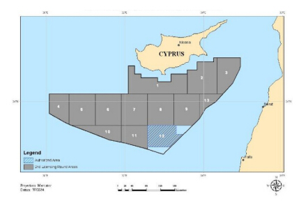
[10] | Government of the Republic of Cyprus. Notice from the Government of the Republic of Cyprus concerning Directive 94/22/EC of the European Parliament and of the Council on the conditions for granting and using authorisations for the prospection, exploration and production of hydrocarbons. Official Journal of the European Union. C38/24, 2012. |
[11] | Government of the Republic of Cyprus, Ministry of Commerce Industry and Tourism. "2nd Licensing round - hydrocarbon exploration". Available: http://www.mcit.gov.cy/mcit/mcit.nsf/dmlhcarbon_en/dmlhcarbon_en?OpenDocument. Cyprus, 2012. |
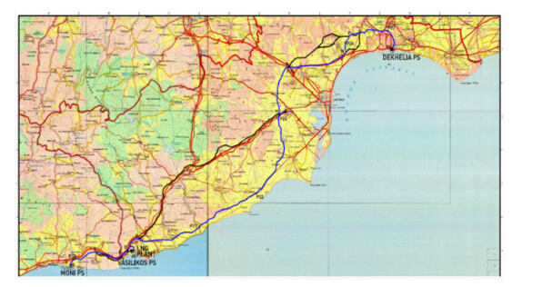
[12] | Natural Gas Public Company (DEFA). Projects: Construction of natural gas pipeline network. Available from: http://www.defa.com.cy/en/projects.html, Cyprus, 2013. |
[13] | European Commission, DG Energy. "Quarterly report on European Gas Markets". Volume 6, issue 1, First quarter, 2013. Available from: http://ec.europa.eu/energy/observatory/gas/doc/20130611_q1_quarterly_report_on_european_gas_markets.pdf |
[14] | European Commission. Emissions trading: Commission adopts decision on Cyprus' national allocation plan for 2008-2012. Press Release, IP-07-1131, Brussels, July 2007. Available from: http://europa.eu/rapid/press-release_IP-07-1131_en.htm |
[15] | European Commision. "The EU emission trading sytem EU ETS". Brussels, 2013. Available from: http://ec.europa.eu/clima/publications/docs/factsheet_ets_2013_en.pdf |
[16] | The European Energy Exchange (EEX). "Market data on Natural Gas Spot prices and trading volumes", Frankfurt, Germany, 2013. Available from: http://www.eex.com/en/EEX |
[17] | Statistical Service of the Cyprus Republic. "Statistical Themes: Energy, Environment". Available from: http://www.mof.gov.cy/mof/cystat/statistics.nsf/energy_environment_81main_gr/energy_environment_81main_gr?OpenForm&sub=1&sel=2 |
[18] | Chasos, C. A., Karagiorgis G. N. and Christodoulou, C. N. (2010) Utilisation of solar/thermal power plants for production of hydrogen with applications in the transportation sector. Proceedings of the 7th Mediterranean Conference and Exhibition on Power Generation, Transmission, Distribution and Energy Conversion (MEDPOWER 2010). Agia Napa, Cyprus, 7-10 November. |
[19] | Cyprus Organisation for Standardisation (CYS) (2008) CYS EN ISO 15403-1:2008: Natural gas — Natural gas for use as compressed fuel for vehicles — Part 1: Designation of the quality. |