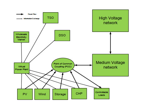
On the whole, the present microgrid constitutes numerous actors in highly decentralized environments and liberalized electricity markets. The networked microgrid system must be capable of detecting electricity price changes and unknown variations in the presence of rare and extreme events. The networked microgrid system comprised of interconnected microgrids must be adaptive and resilient to undesirable environmental conditions such as the occurrence of different kinds of faults and interruptions in the main grid supply. The uncertainties and stochasticity in the load and distributed generation are considered. In this study, we propose resilient energy trading incorporating DC-OPF, which takes generator failures and line outages (topology change) into account. This paper proposes a design of Long Short-Term Memory (LSTM) - soft actor-critic (SAC) reinforcement learning for the development of a platform to obtain resilient peer-to-peer energy trading in networked microgrid systems during extreme events. A Markov Decision Process (MDP) is used to develop the reinforcement learning-based resilient energy trade process that includes the state transition probability and a grid resilience factor for networked microgrid systems. LSTM-SAC continuously refines policies in real-time, thus ensuring optimal trading strategies in rapidly changing energy markets. The LSTM networks have been used to estimate the optimal Q-values in soft actor-critic reinforcement learning. This learning mechanism takes care of the out-of-range estimates of Q-values while reducing the gradient problems. The optimal actions are decided with maximized rewards for peer-to-peer resilient energy trading. The networked microgrid system is trained with the proposed learning mechanism for resilient energy trading. The proposed LSTM-SAC reinforcement learning is tested on a networked microgrid system comprised of IEEE 14 bus systems.
Citation: Desh Deepak Sharma, Ramesh C Bansal. LSTM-SAC reinforcement learning based resilient energy trading for networked microgrid system[J]. AIMS Electronics and Electrical Engineering, 2025, 9(2): 165-191. doi: 10.3934/electreng.2025009
On the whole, the present microgrid constitutes numerous actors in highly decentralized environments and liberalized electricity markets. The networked microgrid system must be capable of detecting electricity price changes and unknown variations in the presence of rare and extreme events. The networked microgrid system comprised of interconnected microgrids must be adaptive and resilient to undesirable environmental conditions such as the occurrence of different kinds of faults and interruptions in the main grid supply. The uncertainties and stochasticity in the load and distributed generation are considered. In this study, we propose resilient energy trading incorporating DC-OPF, which takes generator failures and line outages (topology change) into account. This paper proposes a design of Long Short-Term Memory (LSTM) - soft actor-critic (SAC) reinforcement learning for the development of a platform to obtain resilient peer-to-peer energy trading in networked microgrid systems during extreme events. A Markov Decision Process (MDP) is used to develop the reinforcement learning-based resilient energy trade process that includes the state transition probability and a grid resilience factor for networked microgrid systems. LSTM-SAC continuously refines policies in real-time, thus ensuring optimal trading strategies in rapidly changing energy markets. The LSTM networks have been used to estimate the optimal Q-values in soft actor-critic reinforcement learning. This learning mechanism takes care of the out-of-range estimates of Q-values while reducing the gradient problems. The optimal actions are decided with maximized rewards for peer-to-peer resilient energy trading. The networked microgrid system is trained with the proposed learning mechanism for resilient energy trading. The proposed LSTM-SAC reinforcement learning is tested on a networked microgrid system comprised of IEEE 14 bus systems.

| [1] |
Pudjianto D, Ramsay C, Strbac G (2007) Virtual power plant and system integration of distributed energy resources. IET Renew Power Gen 1: 10‒16. https://doi.org/10.1049/iet-rpg:20060023 doi: 10.1049/iet-rpg:20060023

|
| [2] |
Hanna R, Ghonima M, Kleissl J, Tynan G, Victor DG (2017) Evaluating business models for microgrids: Interactions of technology and policy. Energy Policy 103: 47‒61. https://doi.org/10.1016/j.enpol.2017.01.010 doi: 10.1016/j.enpol.2017.01.010
|
| [3] | Rahman S (2008) Framework for a resilient and environment-friendly microgrid with demand-side participation. Proceedings IEEE Power Eng Soc Gen Meeting—Convers Del Electr Energy 21st Century. https://doi.org/10.1109/PES.2008.4596108 |
| [4] |
Hirsch A, Parag Y, Guerrero J (2018) Microgrids: A review of technologies, key drivers, and outstanding issues. Renewable and Sustainable Energy Reviews 90: 402‒411. https://doi.org/10.1016/j.rser.2018.03.040 doi: 10.1016/j.rser.2018.03.040
|
| [5] |
Mengelkamp E, Gä rttner J, Rock K, Kessler S, Orsini L, Weinhardt C (2018) Designing microgrid energy markets: A case study: The Brooklyn Microgrid. Applied Energy 210: 870‒880. https://doi.org/10.1016/j.apenergy.2017.06.054 doi: 10.1016/j.apenergy.2017.06.054
|
| [6] |
Shahgholian G (2021) A brief review on microgrids: Operation, applications, modeling, and control. Int T Electr Energy Syst 31: e12885. https://doi.org/10.1002/2050-7038.12885 doi: 10.1002/2050-7038.12885
|
| [7] |
Baringo A, L. Baringo L (2016) A stochastic adaptive robust optimization approach for the offering strategy of a virtual power plant. IEEE T Power Syst 32: 3492–3504. https://doi.org/10.1109/TPWRS.2016.2633546 doi: 10.1109/TPWRS.2016.2633546
|
| [8] |
Mishra DK, Ray PK, Li L, Zhang J, Hossain M, Mohanty A (2022) Resilient control based frequency regulation scheme of isolated microgrids considering cyber attack and parameter uncertainties. Applied Energy 306: 118054. https://doi.org/10.1016/j.apenergy.2021.118054 doi: 10.1016/j.apenergy.2021.118054
|
| [9] | Kamal MB, Wei J (2017) Attack- resilient energy management architecture hybrid emergency power system for more-electric aircrafts. 2017 IEEE Power & Energy Society Innovative Smart Grid Technologies Conference (ISGT). https://doi.org/10.1109/ISGT.2017.8085993 |
| [10] |
Hussain A, Bui V, Kim H (2018) A Resilient and Privacy-Preserving Energy Management Strategy for Networked Microgrids. IEEE T Smart Grid 9: 2127‒2139. https://doi.org/10.1109/TSG.2016.2607422 doi: 10.1109/TSG.2016.2607422
|
| [11] |
Khodaei A (2014) Resiliency-oriented microgrid optimal scheduling. IEEE T Smart Grid 5: 1584–1591. https://doi.org/10.1109/TSG.2014.2311465 doi: 10.1109/TSG.2014.2311465
|
| [12] |
Li Y, Li T, Zhang H, Xie X, Sun Q (2022) Distributed resilient Double –Gradient-Descent Based Energy Management Strategy for Multi-Energy System under DoS attacks. IEEE T Netw Sci Eng 9: 2301‒2316. https://doi.org/10.1109/TNSE.2022.3162669 doi: 10.1109/TNSE.2022.3162669
|
| [13] | Liu X (2017) Modelling, analysis, and optimization of interdependent critical infrastructures resilience. Ph. D. thesis, CentraleSupelec. |
| [14] | Mumbere SK, Matsumoto S, Fukuhara A, Bedawy A, Sasaki Y, Zoka Y, et al. (2021) An Energy Management System for Disaster Resilience in Islanded Microgrid Networks. 2021 IEEE PES/IAS Power Africa, 1‒5. https://doi.org/10.1109/PowerAfrica52236.2021.9543282 |
| [15] |
Gholami A, Shekari T, Grijalva S (2019) Proactive management of microgrids for resiliency enhancement: An adaptive robust approach. IEEE T Sustain Energ 10: 470–480. https://doi.org/10.1109/TSTE.2017.2740433 doi: 10.1109/TSTE.2017.2740433
|
| [16] |
Watkins CJ, Dayan P (1992) Q-learning. Machine Learning 8: 279‒292. https://doi.org/10.1007/BF00992698 doi: 10.1007/BF00992698
|
| [17] | Nandy A, Biswas M (2019) Reinforcement learning with open AI Tensor Flow, keras using python, Springer Science (Apress.com). |
| [18] |
Ganesh AH, Xu B (2022) A review of reinforcement learning based energy management systems for electrified powertrains: Progress, challenge, and potential solution. Renew Sust Energ Rev 154: 111833. https://doi.org/10.1016/j.rser.2021.111833 doi: 10.1016/j.rser.2021.111833
|
| [19] |
Zhang T, Sun M, Qiu D, Zhang X, Strbac G, Kang C (2023) A Bayesian Deep Reinforcement Learning-based Resilient Control for Multi-Energy Micro-gird. IEEE T Power Syst 38: 5057‒5072. https://doi.org/10.1109/TPWRS.2023.3233992 doi: 10.1109/TPWRS.2023.3233992
|
| [20] |
Wang Y, Qiu D, Strbac G (2022) Multi-agent deep reinforcement learning for resilience-driven routing and scheduling of mobile energy storage systems. Appl Energ 310: 118575. https://doi.org/10.1016/j.apenergy.2022.118575 doi: 10.1016/j.apenergy.2022.118575
|
| [21] | Chen Y, Heleno M, Moreira A, Gel YR (2023) Topological Graph Convolutional Networks Solutions for Power Distribution Grid Planning. In: Kashima, H., Ide, T., Peng, WC. (eds) Advances in Knowledge Discovery and Data Mining. PAKDD 2023, 123‒134. https://doi.org/10.1007/978-3-031-33374-3_10 |
| [22] |
Zhang B, Hu W, Cao D, Li T, Zhang Z, Chen Z, et al. (2021) Soft actor-critic–based multi-objective optimized energy conversion and management strategy for integrated energy systems with renewable energy. Energ Convers Manage 243: 114381. https://doi.org/10.1016/j.enconman.2021.114381 doi: 10.1016/j.enconman.2021.114381
|
| [23] |
Xu D, Cui Y, Ye J, Cha SW, Li A, Zheng C (2022) A soft actor-critic-based energy management strategy for electric vehicles with hybrid energy storage systems. J Power Sources 524: 231099. https://doi.org/10.1016/j.jpowsour.2022.231099 doi: 10.1016/j.jpowsour.2022.231099
|
| [24] |
Wang S, Diao R, Xu C, Shi D, Wang Z (2021) On Multi-Event Co-Calibration of Dynamic Model Parameters Using Soft Actor-Critic. IEEE T Power Syst 36: 521‒524. https://doi.org/10.1109/TPWRS.2020.3030164 doi: 10.1109/TPWRS.2020.3030164
|
| [25] |
Duan J, Guan Y, Li SE, Ren Y, Sun Q, Cheng B (2022) Distributional Soft Actor-Critic: Off-Policy Reinforcement Learning for Addressing Value Estimation Errors. IEEE T Neur Net Lear Syst33: 6584‒6598. https://doi.org/10.1109/TNNLS.2021.3082568 doi: 10.1109/TNNLS.2021.3082568
|
| [26] |
Zhang Z, Chen Z, Lee WJ (2022) Soft Actor-Critic Algorithm Featured Residential Demand Response Strategic Bidding for Load Aggregators. IEEE T Ind Appl 58: 4298‒4308. https://doi.org/10.1109/TIA.2022.3172068 doi: 10.1109/TIA.2022.3172068
|
| [27] |
Kathirgamanathan A, Mangina E, Finn DP (2021) Development of a Soft Actor-Critic deep reinforcement learning approach for harnessing energy. Energy and AI 5: 100101. https://doi.org/10.1016/j.egyai.2021.100101 doi: 10.1016/j.egyai.2021.100101
|
| [28] |
Ergen T, Kozat SS (2020) Unsupervised Anomaly Detection With LSTM Neural Networks. IEEE T Neur Net Lear Syst 31: 3127‒3141. https://doi.org/10.1109/TNNLS.2019.2935975 doi: 10.1109/TNNLS.2019.2935975
|
| [29] |
Bataineh AA, Kaur D (2021) Immunocomputing-Based Approach for Optimizing the Topologies of LSTM Networks. IEEE Access 9: 78993‒79004. https://doi.org/10.1109/ACCESS.2021.3084131 doi: 10.1109/ACCESS.2021.3084131
|
| [30] |
Zhou Y, Ma Z, Zhang J, Zou S (2022) Data-driven stochastic energy management of multi-energy system using deep reinforcement learning. Energy 261: 125187–125202. https://doi.org/10.1016/j.energy.2022.125187 doi: 10.1016/j.energy.2022.125187
|
| [31] |
Kumar J, Goomer R, Singh AK (2018) Long Short-Term Memory Recurrent Neural Network (LSTM-RNN) Based Workload Forecasting Model For Cloud Datacenters. Procedia Computer Science 125: 676‒682. https://doi.org/10.1016/j.procs.2017.12.087 doi: 10.1016/j.procs.2017.12.087
|
| [32] |
Abbasimehr H, Paki R (2022) Improving time series forecasting using LSTM and attention models. J Amb Intell Human Comput 13: 673–691. https://doi.org/10.1007/s12652-020-02761-x doi: 10.1007/s12652-020-02761-x
|
| [33] |
Liu Q, Long L, Yang Q, Peng H, Wang J, Luo X (2022) LSTM-SNP: A long short-term memory model inspired from spiking neural P systems. Knowledge-Based Systems 235: 107656. https://doi.org/10.1016/j.knosys.2021.107656 doi: 10.1016/j.knosys.2021.107656
|
| [34] |
Moghar A, Hamiche M (2020) Stock Market Prediction Using LSTM Recurrent Neural Network. Procedia Computer Science 170: 1168‒1173. https://doi.org/10.1016/j.procs.2020.03.049 doi: 10.1016/j.procs.2020.03.049
|
| [35] |
Karijadi I, Chou S (2022) A hybrid RF-LSTM based on CEEMDAN for improving the accuracy of building energy consumption prediction. Energy and Buildings 259: 111908. https://doi.org/10.1016/j.enbuild.2022.111908 doi: 10.1016/j.enbuild.2022.111908
|
| [36] |
Zhao L, Mo C, Ma J, Chen Z, Yao C (2022) LSTM-MFCN: A time series classifier based on multi-scale spatial–temporal features. Comput Commun 182: 52‒59. https://doi.org/10.1016/j.comcom.2021.10.036 doi: 10.1016/j.comcom.2021.10.036
|
| [37] |
Ariza I, Tardón LJ, Barbancho AM, De-Torres I, Barbancho I (2022) Bi-LSTM neural network for EEG-based error detection in musicians' performance. Biomed Signal Process Control 78: 103885. https://doi.org/10.1016/j.bspc.2022.103885 doi: 10.1016/j.bspc.2022.103885
|
| [38] |
Karim F, Majumdar, S, Darabi H, Harford S (2019) Multivariate LSTM-FCNs for time series classification. Neural Networks 116: 237‒245. https://doi.org/10.1016/j.neunet.2019.04.014 doi: 10.1016/j.neunet.2019.04.014
|
| [39] |
Saini KK, Sharma P, Mathur HD, Gautam AR, Bansal RC (2024) Techno-economic and Reliability Assessment of an Off-grid Solar-powered Energy System. Appl Energy 371: 123579. https://doi.org/10.1016/j.apenergy.2024.123579 doi: 10.1016/j.apenergy.2024.123579
|
| [40] |
Sharma DD (2024) Asynchronous Blockchain-based Federated Learning for Tokenized Smart Power Contract of Heterogeneous Networked Microgrid System. IET Blockchain 4: 302‒314. https://doi.org/10.1049/blc2.12041 doi: 10.1049/blc2.12041
|
| [41] |
Sharma DD, Singh SN, Lin J (2024) Blockchain-enabled secure and authentic Nash Equilibrium strategies for heterogeneous networked hub of electric vehicle charging stations. Blockchain: Research and Applications 5: 100223. https://doi.org/10.1016/j.bcra.2024.100223 doi: 10.1016/j.bcra.2024.100223
|
| [42] |
Foruzan E, Soh L, Asgarpoor S (2018) Reinforcement Learning Approach for Optimal Distributed Energy Management in a Microgrid. IEEE Trans Power Syst 33: 5749‒5758. https://doi.org/10.1109/TPWRS.2018.2823641 doi: 10.1109/TPWRS.2018.2823641
|
| [43] | Suttan RS, Barto AG (2018) Reinforcement Learning: An introduction, the MIT Press London, England. |


Figures(10) / Tables(2)

Desh Deepak Sharma, Ramesh C Bansal. LSTM-SAC reinforcement learning based resilient energy trading for networked microgrid system[J]. AIMS Electronics and Electrical Engineering, 2025, 9(2): 165-191. doi: 10.3934/electreng.2025009


 DownLoad: