Prediction of diabetic patients in Iraq using binary dragonfly algorithm with long-short term memory neural network

Zaineb M. Alhakeem; Heba Hakim; Ola A. Hasan; Asif Ali Laghari; Awais Khan Jumani; Mohammed Nabil Jasm; Zaineb M. Alhakeem; Heba Hakim; Ola A. Hasan; Asif Ali Laghari; Awais Khan Jumani; Mohammed Nabil Jasm

doi:10.3934/electreng.2023013

AIMS Electronics and Electrical Engineering

2023, Volume 7, Issue 3: 217-230. doi: 10.3934/electreng.2023013

Previous Article Next Article

Research article

Prediction of diabetic patients in Iraq using binary dragonfly algorithm with long-short term memory neural network

1.
Chemical Engineering and Oil Refining Department, Oil and Gas Engineering College, Basrah University for Oil and Gas, Basrah, Iraq
2.
Computer Engineering Department, Engineering College, University of Basrah, Basrah, Iraq
3.
Real Estate Bank of Iraq, Basrah, Iraq
4.
Software college, Shenyang Normal University, Shenyang, China
5.
School of Electronic and Information Engineering, South China University of Technology, Guangzhou, Guangdong, China
6.
Department of Computer Science, ILMA University Karachi, Sindh, Pakistan
7.
Basra Oil Company, Basrah, Iraq
8.
Computer Technology Engineering Department, Iraq University College, Basrah, Iraq

Received: 14 July 2023 Revised: 30 August 2023 Accepted: 04 September 2023 Published: 18 September 2023

Over the past 20 years, there has been a surge of diabetes cases in Iraq. Blood tests administered in the absence of professional medical judgment have allowed for the early detection of diabetes, which will fasten disease detection and lower medical costs. This work focuses on the use of a Long-Short Term Memory (LSTM) neural network for diabetes classification in Iraq. Some medical tests and body features were used as classification features. The most relevant features were selected using the Binary Dragon Fly Algorithm (BDA) Binary version of the selection method because the features either selected or not. To reduce the number of features that are used in prediction, features without effects will be eliminated. This effects the classification accuracy, which is very important in both the computation time of the method and the cost of medical test that the individual will take during annual check ups.This work found out that among 11 features, only five features are most relevant to the disease. These features provide a classification accuracy up to 98% among three classes: diabetic, non diabetic and pre-diabetic.
- diabetes,
- binary dragon fly algorithm,
- long short term memory classifier,
- multi class classification
Citation: Zaineb M. Alhakeem, Heba Hakim, Ola A. Hasan, Asif Ali Laghari, Awais Khan Jumani, Mohammed Nabil Jasm. Prediction of diabetic patients in Iraq using binary dragonfly algorithm with long-short term memory neural network[J]. AIMS Electronics and Electrical Engineering, 2023, 7(3): 217-230. doi: 10.3934/electreng.2023013

Related Papers:

Abstract

Over the past 20 years, there has been a surge of diabetes cases in Iraq. Blood tests administered in the absence of professional medical judgment have allowed for the early detection of diabetes, which will fasten disease detection and lower medical costs. This work focuses on the use of a Long-Short Term Memory (LSTM) neural network for diabetes classification in Iraq. Some medical tests and body features were used as classification features. The most relevant features were selected using the Binary Dragon Fly Algorithm (BDA) Binary version of the selection method because the features either selected or not. To reduce the number of features that are used in prediction, features without effects will be eliminated. This effects the classification accuracy, which is very important in both the computation time of the method and the cost of medical test that the individual will take during annual check ups.This work found out that among 11 features, only five features are most relevant to the disease. These features provide a classification accuracy up to 98% among three classes: diabetic, non diabetic and pre-diabetic.

References

[1]	Iraq diabetes report 2000-2045. Available from: https://www.diabetesatlas.org/data/en/country/96/iq.html
[2]	Tigga NP, Garg S (2023) Speech Emotion Recognition for multiclass classification using Hybrid CNN-LSTM. International Journal of Microsystems and Iot 1: 9–17. https://doi.org/10.5281/zenodo.8158288 doi: 10.5281/zenodo.8158288
[3]	Jaber HA, Rashid MT (2019) HD-sEMG gestures recognition by SVM classifier for controlling prosthesis. Iraqi Journal of Computers, Communications, Control and System Engineering (IJCCCE) 19: 10–19. https://doi.org/10.33103/uot.ijccce.19.1.2 doi: 10.33103/uot.ijccce.19.1.2
[4]	Abgeena A, Garg S (2023) A novel convolution bi-directional gated recurrent unit neural network for emotion recognition in multichannel electroencephalogram signals. Technol Health Care 31: 1215–1234. https://doi.org/10.3233/THC-220458 doi: 10.3233/THC-220458
[5]	Mujumdar A, Vaidehi V (2019) Diabetes prediction using machine learning algorithms. Procedia Computer Science 165: 292–299. https://doi.org/10.1016/j.procs.2020.01.047 doi: 10.1016/j.procs.2020.01.047
[6]	Madan P, Singh V, Chaudhari V, Albagory Y, Dumka A, Singh R, et al. (2022) An optimization-based diabetes prediction model using cnn and bi-directional lstm in real-time environment. Applied Sciences 12: 3989. https://doi.org/10.3390/app12083989 doi: 10.3390/app12083989
[7]	Chang V, Bailey J, Xu QA, Sun Z (2023) Pima indians diabetes mellitus classification based on machine learning (ml) algorithms. Neural Computing and Applications 36: 16157–16173. https://doi.org/10.1007/s00521-022-07049-z doi: 10.1007/s00521-022-07049-z
[8]	Noori NA, Yassin AA (2021) A comparative analysis for diabetic prediction based on machine learning techniques. Journal of Basrah Researches (Sciences) 47.
[9]	Ahamed BS, Arya MS, Nancy AO (2022) Prediction of type-2 diabetes mellitus disease using machine learning classifiers and techniques. Frontiers in Computer Science 4: 835242. https://doi.org/10.1155/2022/9220560 doi: 10.1155/2022/9220560
[10]	Butt UM, Letchmunan S, Ali M, Hassan FH, Baqir A, Sherazi H (2021) Machine learning based diabetes classification and prediction for healthcare applications. Journal of healthcare engineering 2021. https://doi.org/10.1155/2021/9930985
[11]	Zou Q, Qu K, Luo Y, Yin D, Ju Y, Tang H (2018) Predicting diabetes mellitus with machine learning techniques. Frontiers in genetics 9: 515. https://doi.org/10.3389/fgene.2018.00515 doi: 10.3389/fgene.2018.00515
[12]	Naz H, Ahuja S (2020) Deep learning approach for diabetes prediction using pima indian dataset. Journal of Diabetes and Metabolic Disorders 19: 391–403. https://doi.org/10.1007/s40200-020-00520-5 doi: 10.1007/s40200-020-00520-5
[13]	Olisah CC, Smith L, Smith M (2022) Diabetes mellitus prediction and diagnosis from a data preprocessing and machine learning perspective. Comput Meth Prog Bio 220: 106773. https://doi.org/10.1016/j.cmpb.2022.106773 doi: 10.1016/j.cmpb.2022.106773
[14]	Rashid A (2020) Diabetes dataset, Mendeley Data.
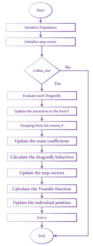
[15]	Mirjalili S (2015) Dragonfly algorithm: A new meta-heuristic optimization technique for solving single-objective, discrete, and multi-objective problems. Neural Comput Appl 27: 1053–1073. https://doi.org/10.1007/s00521-015-1920-1 doi: 10.1007/s00521-015-1920-1
[16]	Mafarja MM, Eleyan D, Jaber I, Hammouri A, Mirjalili S (2017) Binary Dragonfly Algorithm for Feature Selection. 2017 International Conference on New Trends in Computing Sciences (ICTCS), 12–17.
[17]	Alhakeem ZM, Ali RS (2019) Fast channel selection method using crow search algorithm. Proceedings of the International Conference on Information and Communication Technology, 210–214. https://doi.org/10.1145/3321289.3321309
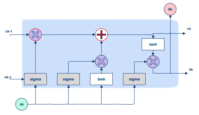
[18]	Hochreiter S, Schmidhuber J (1997) Long Short-Term Memory. Neural Computation 9: 1735–1780. https://doi.org/10.1162/neco.1997.9.8.1735 doi: 10.1162/neco.1997.9.8.1735
[19]	Dalianis H (2018) Evaluation Metrics and Evaluation, Cham: Springer International Publishing. https://doi.org/10.1007/978-3-319-78503-5_6

Reader Comments

Your name:*

Email:*
© 2023 the Author(s), licensee AIMS Press. This is an open access article distributed under the terms of the Creative Commons Attribution License (http://creativecommons.org/licenses/by/4.0)