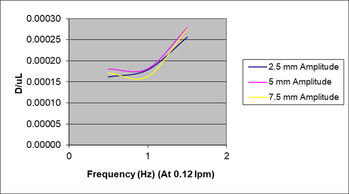
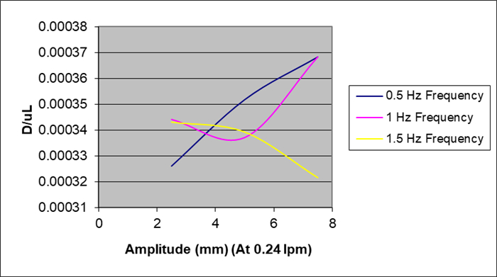
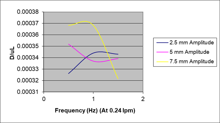
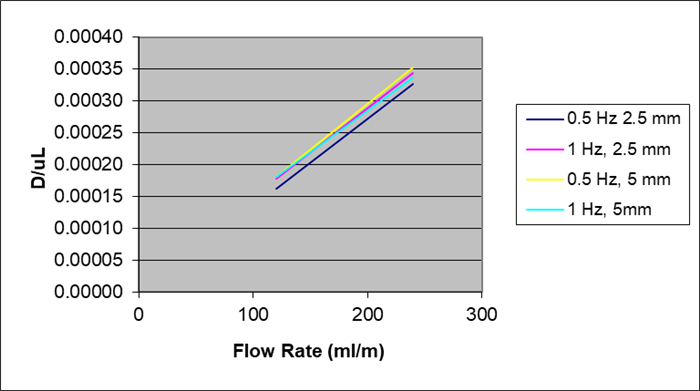
Hydrogen is an environmentally attractive transportation fuel that can replace fossil fuels. The iodine-sulfur (I-S) thermo-chemical process involves three reaction steps. The Bunsen reaction is one of the main reaction steps of I-S process and plays an important role in defining overall process efficiency. Different types of reactors are being studied, including the oscillatory baffle Bunsen reactor. The reactor selection is based on process intensification and process integration, i.e., reaction and separation in the single equipment. Simulations are performed for two-dimensional cases by solving incompressible Navier-Stokes equations along with continuity equation, the geometry chosen is of single section in the column and diameter of 50 mm and baffle spacing of 50, 75,100 mm i.e. 1, 1.5 and 2 times the diameter of column and baffle free area 22%. The residence time distribution experiments are carried out in a metallic reactor with NaCl as a tracer operated at different frequencies, amplitudes and flow rates. D/uL is evaluated from experimental curves. The power per unit mass is compared for oscillatory baffled column and stirred tank for a semi-batch process. From the numerical simulations, good eddy interactions are present at higher frequencies and amplitudes and at a baffle spacing of 1.5 times the diameter of the column. Residence time distribution analysis gives a lower dispersion number at medium frequencies and higher amplitudes with constant flow rate. If the flow rates are high, then it is better to operate at higher frequencies and amplitudes to achieve plug flow behavior. Power per unit mass is less for oscillatory baffle column compared to the stirred tank of given configuration. With better mixing performance and less power per unit volume, the oscillatory baffle column is a good alternative to other columns.
Citation: V Nafees Ahmed, A Shriniwas Rao. Performance evaluation of oscillatory baffle Bunsen reactor in iodine sulfur thermochemical process for hydrogen production[J]. Clean Technologies and Recycling, 2023, 3(4): 267-282. doi: 10.3934/ctr.2023017
Hydrogen is an environmentally attractive transportation fuel that can replace fossil fuels. The iodine-sulfur (I-S) thermo-chemical process involves three reaction steps. The Bunsen reaction is one of the main reaction steps of I-S process and plays an important role in defining overall process efficiency. Different types of reactors are being studied, including the oscillatory baffle Bunsen reactor. The reactor selection is based on process intensification and process integration, i.e., reaction and separation in the single equipment. Simulations are performed for two-dimensional cases by solving incompressible Navier-Stokes equations along with continuity equation, the geometry chosen is of single section in the column and diameter of 50 mm and baffle spacing of 50, 75,100 mm i.e. 1, 1.5 and 2 times the diameter of column and baffle free area 22%. The residence time distribution experiments are carried out in a metallic reactor with NaCl as a tracer operated at different frequencies, amplitudes and flow rates. D/uL is evaluated from experimental curves. The power per unit mass is compared for oscillatory baffled column and stirred tank for a semi-batch process. From the numerical simulations, good eddy interactions are present at higher frequencies and amplitudes and at a baffle spacing of 1.5 times the diameter of the column. Residence time distribution analysis gives a lower dispersion number at medium frequencies and higher amplitudes with constant flow rate. If the flow rates are high, then it is better to operate at higher frequencies and amplitudes to achieve plug flow behavior. Power per unit mass is less for oscillatory baffle column compared to the stirred tank of given configuration. With better mixing performance and less power per unit volume, the oscillatory baffle column is a good alternative to other columns.

| [1] |
Jain IP (2009) Hydrogen the fuel for 21st century. Int J Hydrogen Energy 34: 7368–7378. https://doi.org/10.1016/j.ijhydene.2009.05.093 doi: 10.1016/j.ijhydene.2009.05.093

|
| [2] |
Beghi GE (1986) A decade of research on thermochemical hydrogen at the Joint Research Centre, Ispra. Int J Hydrogen Energy 11: 761–771. https://doi.org/10.1016/0360-3199(86)90172-2 doi: 10.1016/0360-3199(86)90172-2
|
| [3] |
Lee BJ, No HC, Yoon HJ, et al. (2008) An optimal operating window for the Bunsen process in the I–S thermochemical cycle. Int J Hydrogen Energy 33: 2200–2210. https://doi.org/10.1016/j.ijhydene.2008.02.045 doi: 10.1016/j.ijhydene.2008.02.045
|
| [4] |
Ahmed VN, Rao AS, Sujeesh S, et al. (2018) Evaluation of Bunsen reaction at elevated temperature and high pressure in continuous co-current reactor in iodine-sulfur thermochemical process. Int J Hydrogen Energy 43: 8190–8197. https://doi.org/10.1016/j.ijhydene.2018.03.098 doi: 10.1016/j.ijhydene.2018.03.098
|
| [5] |
Ahmed VN, Rao AS, Sujeesh S, et al. (2017) Role of operating conditions on cross contamination of products of the Bunsen reaction in iodine-sulfur process for production of hydrogen. Int J Hydrogen Energy 42: 29101–29106. https://doi.org/10.1016/j.ijhydene.2017.09.133 doi: 10.1016/j.ijhydene.2017.09.133
|
| [6] | Norman JH, Besenbruch GE, Brown LC, et al., Thermochemical water-splitting cycle, bench-scale investigations, and process engineering, final report for the period February 1977 through December 31, 1981. GA-A16713, 1982. Available from: https://www.osti.gov/biblio/5063416. |
| [7] | Richardson JF (2002) Coulson & Richardson's Chemical Engineering Design, Amsterdam: Elsevier. |
| [8] |
Ni X (1995) A study of fluid dispersion in oscillatory flow through a baffled tube. J Chem Technol Biotechnol 64: 165–174. https://doi.org/10.1002/jctb.280640209 doi: 10.1002/jctb.280640209
|
| [9] |
Stonestreet P, Harvey AP (2002) A mixing-based design methodology for continuous oscillatory flow reactors. Chem Eng Res Des 80: 31–44. https://doi.org/10.1205/026387602753393204 doi: 10.1205/026387602753393204
|
| [10] |
Torab-Mostaedi M, Safdari J (2009) Mass transfer coefficients in a pulsed packed extraction column. Chem Eng Process Process Intensif 48: 1321–1326. https://doi.org/10.1016/j.cep.2009.06.002 doi: 10.1016/j.cep.2009.06.002
|
| [11] |
Ni X, Mackley MR, Harvey AP (2003) Mixing through oscillations and pulsations—a guide to achieving process enhancements in the chemical and process industries. Chem Eng Res Des 81: 373–383. https://doi.org/10.1205/02638760360596928 doi: 10.1205/02638760360596928
|
| [12] |
McGlone T, Briggs NEB, Clark CA, et al. (2015) Oscillatory flow reactors (OFRs) for continuous manufacturing and crystallization. Org Process Res Dev 19: 1186–1202. https://doi.org/10.1021/acs.oprd.5b00225 doi: 10.1021/acs.oprd.5b00225
|
| [13] |
Ni X, Gough P (1997) On the discussion of the dimensionless groups governing oscillatory flow in a baffled tube. Chem Eng Sci 52: 3209–3212. https://doi.org/10.1016/S0009-2509(97)00104-8 doi: 10.1016/S0009-2509(97)00104-8
|
| [14] |
Mackley MR, Ni X (1991) Mixing and dispersion in a baffled tube for steady laminar and pulsatile flow. Chem Eng Sci 46: 3139–3151. https://doi.org/10.1016/0009-2509(91)85017-R doi: 10.1016/0009-2509(91)85017-R
|
| [15] | Levenspiel O (1998) Chemical Reaction Engineering, 3 Eds., Hoboken: John Wiley & Sons. |
| [16] |
Brunold CR, Hunns JCB, Mackley MR, et al. (1989) Experimental observations on flow patterns and energy losses for oscillatory flow in ducts containing sharp edges. Chem Eng Sci 44: 1227–1244. https://doi.org/10.1016/0009-2509(89)87022-8 doi: 10.1016/0009-2509(89)87022-8
|
| [17] | COMSOL, COMSOL Multiphysics. COMSOL, n.d. Available from: https://doc.comsol.com/5.5/doc/com.comsol.help.comsol/COMSOL_ReferenceManual.pdf. |
| [18] |
Zheng M, Mackley M (2008) The axial dispersion performance of an oscillatory flow meso-reactor with relevance to continuous flow operation. Chem Eng Sci 63: 1788–1799. https://doi.org/10.1016/j.ces.2007.12.020 doi: 10.1016/j.ces.2007.12.020
|
| [19] | McCabe WL, Smith JC, Harriott P (1993) Unit Operations of Chemical Engineering, 5 Eds., New York: McGraw-hill. |
| [20] | Baird MH, Stonestreet P (1995) Energy-dissipation in oscillatory flow within a baffled tube. Chem Eng Res Des 73: 503–511. |
Figures(16)
V Nafees Ahmed, A Shriniwas Rao. Performance evaluation of oscillatory baffle Bunsen reactor in iodine sulfur thermochemical process for hydrogen production[J]. Clean Technologies and Recycling, 2023, 3(4): 267-282. doi: 10.3934/ctr.2023017


 DownLoad: