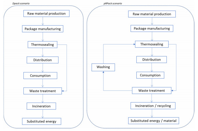
To limit the huge damage caused by plastic pollution, major changes need to be made in the food and beverage packaging sector. In this context, a new packaging system for dry-cured ham slices, containing natural antioxidants, was developed; it consists of a reusable polymer tray sealed with disposable polymer film. The life cycle of the packaging was assessed to compare its environmental impacts with a reference disposable packaging system already in use. The life cycle assessment was performed in accordance with the ISO 14040-14044 series; the system was model using the Gabi software and the ILCD PEF method was used to evaluate the impacts. The functional unit chosen was to pack 1000 batches of 4 slices of dry-cured ham in France. Three packaging scenarios were compared: a reference disposable packaging system, incinerated at end of life; the partially reusable packaging, recycled at end of life and the same partially reusable packaging, incinerated at end of life. The study of the relative impacts of each scenario revealed that for the reference packaging, the production of the tray was the highest-impact stage. With the reusable packaging, the highest-impact stages were the thermosealing process and the production of the trays and films. A significant reduction in all impacts was observed with the use of the reusable packaging. Sensitivity analysis was carried out to study the influence of the breakage rate of the tray during reuse and the number of reuse cycles of the tray. Except for freshwater resource depletion, the reusable packaging had lower environmental impacts even with a high tray breakage rate or a low number of reuses. This paper demonstrates the interest of this reusable and recyclable food contact packaging to lower the environmental footprint of packaging; the reuse and recycling stages now need to be tested in real situations for the packaging prototype to confirm the feasibility of the reuse process.
Citation: Joana Beigbeder, Ahmed Allal, Nathalie Robert. Ex-ante life cycle assessment of a partially reusable packaging system for dry-cured ham slices[J]. Clean Technologies and Recycling, 2022, 2(3): 119-135. doi: 10.3934/ctr.2022007
To limit the huge damage caused by plastic pollution, major changes need to be made in the food and beverage packaging sector. In this context, a new packaging system for dry-cured ham slices, containing natural antioxidants, was developed; it consists of a reusable polymer tray sealed with disposable polymer film. The life cycle of the packaging was assessed to compare its environmental impacts with a reference disposable packaging system already in use. The life cycle assessment was performed in accordance with the ISO 14040-14044 series; the system was model using the Gabi software and the ILCD PEF method was used to evaluate the impacts. The functional unit chosen was to pack 1000 batches of 4 slices of dry-cured ham in France. Three packaging scenarios were compared: a reference disposable packaging system, incinerated at end of life; the partially reusable packaging, recycled at end of life and the same partially reusable packaging, incinerated at end of life. The study of the relative impacts of each scenario revealed that for the reference packaging, the production of the tray was the highest-impact stage. With the reusable packaging, the highest-impact stages were the thermosealing process and the production of the trays and films. A significant reduction in all impacts was observed with the use of the reusable packaging. Sensitivity analysis was carried out to study the influence of the breakage rate of the tray during reuse and the number of reuse cycles of the tray. Except for freshwater resource depletion, the reusable packaging had lower environmental impacts even with a high tray breakage rate or a low number of reuses. This paper demonstrates the interest of this reusable and recyclable food contact packaging to lower the environmental footprint of packaging; the reuse and recycling stages now need to be tested in real situations for the packaging prototype to confirm the feasibility of the reuse process.

| [1] | Horton AA (2022) Plastic pollution: When do we know enough? J Hazard Mater 422: 126885. |
| [2] |
Iroegbu AOC, Ray SS, Mbarane V, et al. (2021) Plastic Pollution: A Perspective on Matters Arising: Challenges and Opportunities. ACS Omega 6: 19343-19355. https://doi.org/10.1016/j.jhazmat.2021.126885 doi: 10.1016/j.jhazmat.2021.126885

|
| [3] | Ellen MacArthur Foundation, The New Plastics Economy—Rethinking the future of plastics, 2016. Available form: https://ellenmacarthurfoundation.org/the-new-plastics-economy-rethinking-the-future-of-plastics-and-catalysing. https://doi.org/10.1021/acsomega.1c02760. |
| [4] |
Phelan AA, Meissner K, Humphrey J, et al. (2022) Plastic pollution and packaging: Corporate commitments and actions from the food and beverage sector. J Clean Prod 331: 129827. https://doi.org/10.1016/j.jclepro.2021.129827 doi: 10.1016/j.jclepro.2021.129827
|
| [5] |
Persson L, Carney Almroth BM, Collins CD, et al. (2022) Outside the safe operating space of the planetary boundary for novel entities. Environ Sci Technol 56: 1510-1521. https://doi.org/10.1021/acs.est.1c04158 doi: 10.1021/acs.est.1c04158
|
| [6] | Karlsson T, Brosché S, Alidoust M, et al. (2021) Plastic pellets found on beaches all over the world contain toxic chemicals. Available form: https://ipen.org/documents/plastic-pellets-found-beaches-all-over-world-contain-toxic-chemicals. |
| [7] |
Wiesinger H, Wang Z, Hellweg S (2021) Deep dive into plastic monomers, additives, and processing aids. Environ Sci Technol 55: 9339-9351. https://doi.org/10.1021/acs.est.1c00976 doi: 10.1021/acs.est.1c00976
|
| [8] |
Senko JF, Nelms SE, Reavis JL, et al. (2020) Understanding individual and population-level effects of plastic pollution on marine megafauna. Endanger Species Res 43: 234-252. https://doi.org/10.3354/esr01064 doi: 10.3354/esr01064
|
| [9] |
Gall SC, Thompson RC (2015) The impact of debris on marine life. Mar Pollut Bull 92: 170-179. https://doi.org/10.1016/j.marpolbul.2014.12.041 doi: 10.1016/j.marpolbul.2014.12.041
|
| [10] |
Kasavan S, Yusoff S, Rahmat Fakri MF, et al. (2021) Plastic pollution in water ecosystems: A bibliometric analysis from 2000 to 2020. J Clean Prod 313: 127946. https://doi.org/10.1016/j.jclepro.2021.127946 doi: 10.1016/j.jclepro.2021.127946
|
| [11] |
Kurniawan SB, Said NSM, Imron MF, et al. (2021) Microplastic pollution in the environment: Insights into emerging sources and potential threats. Environ Technol Innov 23: 101790. https://doi.org/10.1016/j.eti.2021.101790 doi: 10.1016/j.eti.2021.101790
|
| [12] |
Jaiswal KK, Dutta S, Banerjee I, et al. (2022) Impact of aquatic microplastics and nanoplastics pollution on ecological systems and sustainable remediation strategies of biodegradation and photodegradation. Sci Total Environ 806: 151358. https://doi.org/10.1016/j.scitotenv.2021.151358 doi: 10.1016/j.scitotenv.2021.151358
|
| [13] |
Fusi A, Guidetti R, Benedetto G (2014) Delving into the environmental aspect of a Sardinian white wine: From partial to total life cycle assessment. Sci Total Environ 472: 989-1000. https://doi.org/10.1016/j.scitotenv.2013.11.148 doi: 10.1016/j.scitotenv.2013.11.148
|
| [14] |
Gazulla C, Raugei M, Fullana-i-Palmer P (2010) Taking a life cycle look at crianza wine production in Spain: Where are the bottlenecks? Int J Life Cycle Assess 15: 330-337. https://doi.org/10.1007/s11367-010-0173-6 doi: 10.1007/s11367-010-0173-6
|
| [15] |
Manfredi M, Vignali G (2014) Life cycle assessment of a packaged tomato puree: A comparison of environmental impacts produced by different life cycle phases. J Clean Prod 73: 275-284. https://doi.org/10.1016/j.jclepro.2013.10.010 doi: 10.1016/j.jclepro.2013.10.010
|
| [16] |
Pasqualino J, Meneses M, Castells F (2011) The carbon footprint and energy consumption of beverage packaging selection and disposal. J Food Eng 103: 357-365. https://doi.org/10.1016/j.jfoodeng.2010.11.005 doi: 10.1016/j.jfoodeng.2010.11.005
|
| [17] |
Louis D, Lombart C, Durif F (2021) Packaging-free products: A lever of proximity and loyalty between consumers and grocery stores. J Retail Consum Serv 60: 102499. https://doi.org/10.1016/j.jretconser.2021.102499 doi: 10.1016/j.jretconser.2021.102499
|
| [18] |
Flury M, Narayan R (2021) Biodegradable plastic as an integral part of the solution to plastic waste pollution of the environment. Curr Opin Green Sustain Chem 30: 100490. https://doi.org/10.1016/j.cogsc.2021.100490 doi: 10.1016/j.cogsc.2021.100490
|
| [19] |
Silva DAL, Renó GWS, Sevegnani G, et al. (2013) Comparison of disposable and returnable packaging: A case study of reverse logistics in Brazil. J Clean Prod 47: 377-387. https://doi.org/10.1016/j.jclepro.2012.07.057 doi: 10.1016/j.jclepro.2012.07.057
|
| [20] |
Coelho PM, Corona B, ten Klooster R, et al. (2020) Sustainability of reusable packaging-Current situation and trends. Resour Conserv Recycl X 6: 100037. https://doi.org/10.1016/j.rcrx.2020.100037 doi: 10.1016/j.rcrx.2020.100037
|
| [21] | European Union, Directive 2006/12/EC of the European parliament and of the council of 5 April 2006 on waste. OJEU, 2006. Available form: https://eur-lex.europa.eu/legal-content/EN/TXT/PDF/?uri=CELEX:32006L0012&from=RO. |
| [22] | The European Parliament and the Council of the European Union, Directive (EU) 2018/852 of the European Parliament and of the Council of 30 May 2018 amending Directive 94/62/EC on packaging and packaging waste, 2018. Available form: http://data.europa.eu/eli/dir/2018/852/oj. |
| [23] |
Fogt Jacobsen L, Pedersen S, Thøgersen J (2022) Drivers of and barriers to consumers' plastic packaging waste avoidance and recycling—A systematic literature review. Waste Manage 141: 63-78. https://doi.org/10.1016/j.wasman.2022.01.021 doi: 10.1016/j.wasman.2022.01.021
|
| [24] |
Hesser F (2015) Environmental advantage by choice: Ex-ante LCA for a new Kraft pulp fibre reinforced polypropylene composite in comparison to reference materials. Compos Part B-Eng 79: 197-203. https://doi.org/10.1016/j.compositesb.2015.04.038 doi: 10.1016/j.compositesb.2015.04.038
|
| [25] | European Commission, Circular Plastics Alliance, 2022. Available from: https://ec.europa.eu/growth/industry/strategy/industrial-alliances/circular-plastics-alliance_en. |
| [26] | ISO 14040: 2006(en): Environmental management—life cycle assessment—Principles and framework. The International Organization for Standardization, 2006. Available from: https://www.iso.org/obp/ui#iso:std:iso:14040:ed-2:v1:en. |
| [27] | ISO 14044: 2006: Environmental management—Life cycle assessment—Requirements and guidelines. The International Organization for Standardization, 2006. Available from: https://www.iso.org/obp/ui/#iso:std:iso:14044:ed-1:v1:en. |
| [28] | Camps-Posino L, Batlle-Bayer L, Bala A, et al. (2021) Potential climate benefits of reusable packaging in food delivery services. A Chinese case study. Sci Total Environ 794: 148570. https://doi.org/10.1016/j.scitotenv.2021.148570 |
| [29] |
Postacchini L, Mazzuto G, Paciarotti C, et al. (2018) Reuse of honey jars for healthier bees: Developing a sustainable honey jars supply chain through the use of LCA. J Clean Prod 177: 573-588. https://doi.org/10.1016/j.jclepro.2017.12.240 doi: 10.1016/j.jclepro.2017.12.240
|
| [30] |
Accorsi R, Cascini A, Cholette S, et al. (2014) Economic and environmental assessment of reusable plastic containers: A food catering supply chain case study. Int J Prod Econ 152: 88-101. https://doi.org/10.1016/j.ijpe.2013.12.014 doi: 10.1016/j.ijpe.2013.12.014
|
| [31] |
Arunan I, Crawford RH (2021) Greenhouse gas emissions associated with food packaging for online food delivery services in Australia. Resour Conserv Recy 168: 105299. https://doi.org/10.1016/j.resconrec.2020.105299 doi: 10.1016/j.resconrec.2020.105299
|
| [32] |
Tamburini E, Costa S, Summa D, et al. (2021) Plastic (PET) vs bioplastic (PLA) or refillable aluminium bottles—What is the most sustainable choice for drinking water? A life-cycle (LCA) analysis. Environ Res 196: 110974. https://doi.org/10.1016/j.envres.2021.110974 doi: 10.1016/j.envres.2021.110974
|
| [33] |
Sazdovski I, Bala A, Fullana-i-Palmer P (2021) Linking LCA literature with circular economy value creation: A review on beverage packaging. Sci Total Environ 771: 145322. https://doi.org/10.1016/j.scitotenv.2021.145322 doi: 10.1016/j.scitotenv.2021.145322
|
| [34] | Ligthart TN, Ansems AMM (2007) Single use cups or reusable (coffee) drinking systems: an environmental comparison. Available form: http://www.bekerrecycling.nl/nl/file/20110104172024/3/tno-eng.pdf. |
| [35] |
Changwichan K, Gheewala SH (2020) Choice of materials for takeaway beverage cups towards a circular economy. Sustain Prod Consum 22: 34-44. https://doi.org/10.1016/j.spc.2020.02.004 doi: 10.1016/j.spc.2020.02.004
|
| [36] |
Gallego-Schmid A, Mendoza JMF, Azapagic A (2019) Environmental impacts of takeaway food containers. J Clean Prod 211: 417-427. https://doi.org/10.1016/j.jclepro.2018.11.220 doi: 10.1016/j.jclepro.2018.11.220
|
| [37] |
Cottafava D, Costamagna M, Baricco M, et al. (2021) Assessment of the environmental break-even point for deposit return systems through an LCA analysis of single-use and reusable cups. Sustain Prod Consum 27: 228-241. https://doi.org/10.1016/j.spc.2020.11.002 doi: 10.1016/j.spc.2020.11.002
|
| [38] |
Buyle M, Audenaert A, Billen P, et al. (2019) The future of ex-ante LCA? Lessons learned and practical recommendations. Sustain 11: 5456. https://doi.org/10.3390/su11195456 doi: 10.3390/su11195456
|
| [39] | Issart A (2019) Potential of natural antioxidants for the stabilization of polymers for food packaging and the development of methods for evaluating their migration[PhD's thesis]. Université de Pau et des Pays de l'Adour, France. |
| [40] | Allal AM, Issart A (2021) Patent material for food packaging and method for the preparation thereof. European Patent Office, WO/2020/260829. Available form: https://patentscope.wipo.int/search/en/detail.jsf?docId=WO2020260829. |
| [41] | Shonfield P (2008) LCA of management options for mixed waste plastics. Available form: https://silo.tips/download/final-report-lca-of-management-options-for-mixed-waste-plastics. |
| [42] |
Krehula LK, Siročić AP, Dukić M, et al. (2012) Cleaning efficiency of poly (ethylene terephthalate) washing procedure in recycling process. J Elastom Plast 45: 429-444. https://doi.org/10.1177/0095244312457798 doi: 10.1177/0095244312457798
|
| [43] | Doka G (2003) Life cycle inventories of waste treatment services. Available form: https://www.doka.ch/13_I_WasteTreatmentGeneral.pdf. |
| [44] | European Commission, Product environmental footprint category rules guidance—version 6.3, 2018. Available form: https://ec.europa.eu/environment/eussd/smgp/pdf/PEFCR_guidance_v6.3.pdf. |


Figures(8) / Tables(3)
Joana Beigbeder, Ahmed Allal, Nathalie Robert. Ex-ante life cycle assessment of a partially reusable packaging system for dry-cured ham slices[J]. Clean Technologies and Recycling, 2022, 2(3): 119-135. doi: 10.3934/ctr.2022007


 DownLoad: