By injecting a string of spinors within a membrane, it becomes sensitive to external magnetic fields. Without external magnetic fields, half of the spinors in this string have opposite spins with respect to the other half and become paired with them within membranes. However, any external magnetic field could have a direct effect on this system because a magnetic field could make all spinors parallel. According to the exclusion principle, parallel spinors repel each other and go away. Consequently, they force the molecular membrane to grow. By removing external fields, this molecule or membrane returns to its initial size. An injected string of spinors could be designed so that this molecule or membrane is sensitive only to some frequencies. Particularly, membranes could be designed to respond to low frequencies below 60 Hz. Even in some conditions, frequencies should be lower than 20 Hz. Higher frequencies may destroy the structure of membranes. Although, by using some more complicated mechanisms, some membranes could be designed to respond to higher frequencies. Thus, a type of intelligence could be induced into a molecule or membrane such that it becomes able to diagnose special frequencies of waves and responses. We tested the model for milk molecules like fat, vesicles, and microbial ones under a 1000x microscope and observed that it works. Thus, this technique could be used to design intelligent drug molecules. Also, this model may give good reasons for observing some signatures of water memory by using the physical properties of spinors.
Citation: Massimo Fioranelli, Alireza Sepehri, Ilyas Khan, Phoka C. Rathebe. Induction of intelligence into molecules by using spinor radiation: an alternative to water memory[J]. AIMS Biophysics, 2023, 10(2): 247-257. doi: 10.3934/biophy.2023016
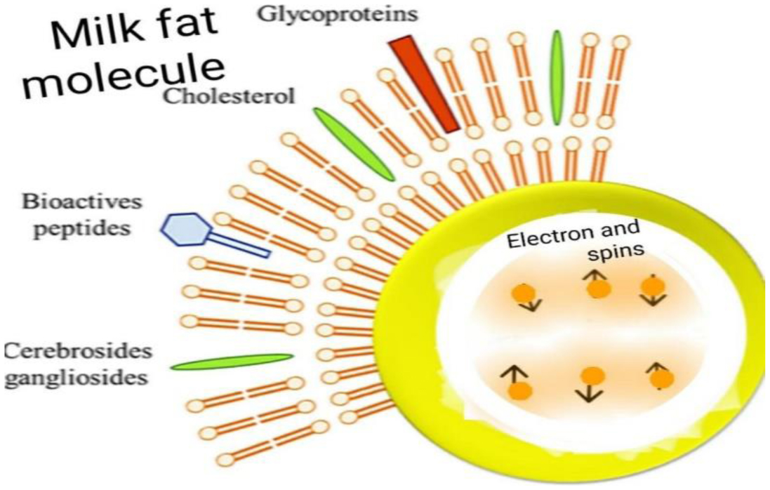
By injecting a string of spinors within a membrane, it becomes sensitive to external magnetic fields. Without external magnetic fields, half of the spinors in this string have opposite spins with respect to the other half and become paired with them within membranes. However, any external magnetic field could have a direct effect on this system because a magnetic field could make all spinors parallel. According to the exclusion principle, parallel spinors repel each other and go away. Consequently, they force the molecular membrane to grow. By removing external fields, this molecule or membrane returns to its initial size. An injected string of spinors could be designed so that this molecule or membrane is sensitive only to some frequencies. Particularly, membranes could be designed to respond to low frequencies below 60 Hz. Even in some conditions, frequencies should be lower than 20 Hz. Higher frequencies may destroy the structure of membranes. Although, by using some more complicated mechanisms, some membranes could be designed to respond to higher frequencies. Thus, a type of intelligence could be induced into a molecule or membrane such that it becomes able to diagnose special frequencies of waves and responses. We tested the model for milk molecules like fat, vesicles, and microbial ones under a 1000x microscope and observed that it works. Thus, this technique could be used to design intelligent drug molecules. Also, this model may give good reasons for observing some signatures of water memory by using the physical properties of spinors.

| [1] |
Humphreys LG (1979) The construct of general intelligence. Intelligence 3: 105-120. https://psycnet.apa.org/doi/10.1016/0160-2896(79)90009-6 
|
| [2] |
Colom R, Karama S, Jung RE, et al. (2022) Human intelligence and brain networks. Dialogues Clin Neuro 12: 489-501. https://doi.org/10.31887/DCNS.2010.12.4/rcolom
|
| [3] |
Salovey P, Mayer JD (1990) Emotional intelligence. Imagin Cogn Pers 9: 185-211. https://psycnet.apa.org/doi/10.2190/DUGG-P24E-52WK-6CDG
|
| [4] |
Wissner-Gross AD, Freer CE (2013) Causal entropic forces. Phys Rev Lett 110: 168702. https://doi.org/10.1103/PhysRevLett.110.168702
|
| [5] |
Goh CH, Nam HG, Park YS (2003) Stress memory in plants. Plant J 36: 240-255. https://doi.org/10.1046/j.1365-313X.2003.01872.x
|
| [6] |
Ford BJ (2017) Cellular intelligence: microphenomenology and the realities of being. Prog Biophys Mol Bio 131: 273-287. https://doi.org/10.1016/j.pbiomolbio.2017.08.012
|
| [7] | Russell SJ, Norvig P Artificial Intelligence: A Modern Approach (2003). |
| [8] |
Scassellati B (2002) Theory of mind for a humanoid robot. Auton Robot 12: 13-24. https://doi.org/10.1023/A:1013298507114
|
| [9] |
Svítek M (2022) Emergent intelligence in generalized pure quantum systems. Computation 10: 88. https://doi.org/10.3390/computation10060088
|
| [10] |
Li W, Enamoto LM, Li DL, et al. (2022) New directions for artificial intelligence: human, machine, biological, and quantum intelligence. Front Inform Technol Electron Eng 23: 984-990. https://doi.org/10.1631/FITEE.2100227
|
| [11] |
Montagniet L, Aissa J, Ferris S, et al. (2009) Electromagnetic signals are produced by aqueous nanostructures derived from bacterial DNA sequences. Interdiscip Sci Comput Life Sci 1: 81-90. https://doi.org/10.1007/s12539-009-0036-7
|
| [12] |
Montagnier L, Del Giudice E, Aïssa J, et al. (2015) Transduction of DNA information through water and electromagnetic waves. Electromagn Biol Med 34: 106-112. https://doi.org/10.3109/15368378.2015.1036072
|
| [13] | Benveniste J, Aissa J, Guillonnet D (1999) The molecular signal is not functional in the absence of informed water. FASEB J 13: A163. |
| [14] |
Jerman I, Ružič R, Krašovec R, et al. (2005) Electrical transfer of molecule information into water, its storage, and bioeffects on plants and bacteria. Electromagn Biol Med 24: 341-353. https://doi.org/10.1080/15368370500381620
|
| [15] |
Bruza PD, Wang Z, Busemeyer JR (2015) Quantum cognition: a new theoretical approach to psychology. Trends Cogn Sci 19: 383-393. https://doi.org/10.1016/j.tics.2015.05.001
|
| [16] |
Liu L, Zhang Y, Wu S, et al. (2018) Water memory effects and their impacts on global vegetation productivity and resilience. Sci Rep 8: 2962. https://doi.org/10.1038/s41598-018-21339-4
|
| [17] |
Colic M, Morse D (1999) The elusive mechanism of the magnetic ‘memory’of water. Colloid Surf A Physicochem Eng Aspects 154: 167-174. https://doi.org/10.1016/S0927-7757(98)00894-2
|
| [18] |
Thomas Y (2007) The history of the memory of water. Homeopathy 96: 151-157. https://doi.org/10.1016/j.homp.2007.03.006
|


Figures(12)

Massimo Fioranelli, Alireza Sepehri, Ilyas Khan, Phoka C. Rathebe. Induction of intelligence into molecules by using spinor radiation: an alternative to water memory[J]. AIMS Biophysics, 2023, 10(2): 247-257. doi: 10.3934/biophy.2023016


 DownLoad: