Similarity of epidemic spreading and information network connectivity mechanisms demonstrated by analysis of two probabilistic models

Into Almiala; Vesa Kuikka; Into Almiala; Vesa Kuikka

doi:10.3934/biophy.2023011

AIMS Biophysics

2023, Volume 10, Issue 2: 173-183. doi: 10.3934/biophy.2023011

Previous Article Next Article

Letter Special Issues

Similarity of epidemic spreading and information network connectivity mechanisms demonstrated by analysis of two probabilistic models

Into Almiala ,
Vesa Kuikka ^,

Finnish Defence Research Agency, Tykkikentäntie 1, PO BOX 10, 11311 Riihimäki, Finland

Received: 12 January 2023 Revised: 04 April 2023 Accepted: 19 April 2023 Published: 25 April 2023

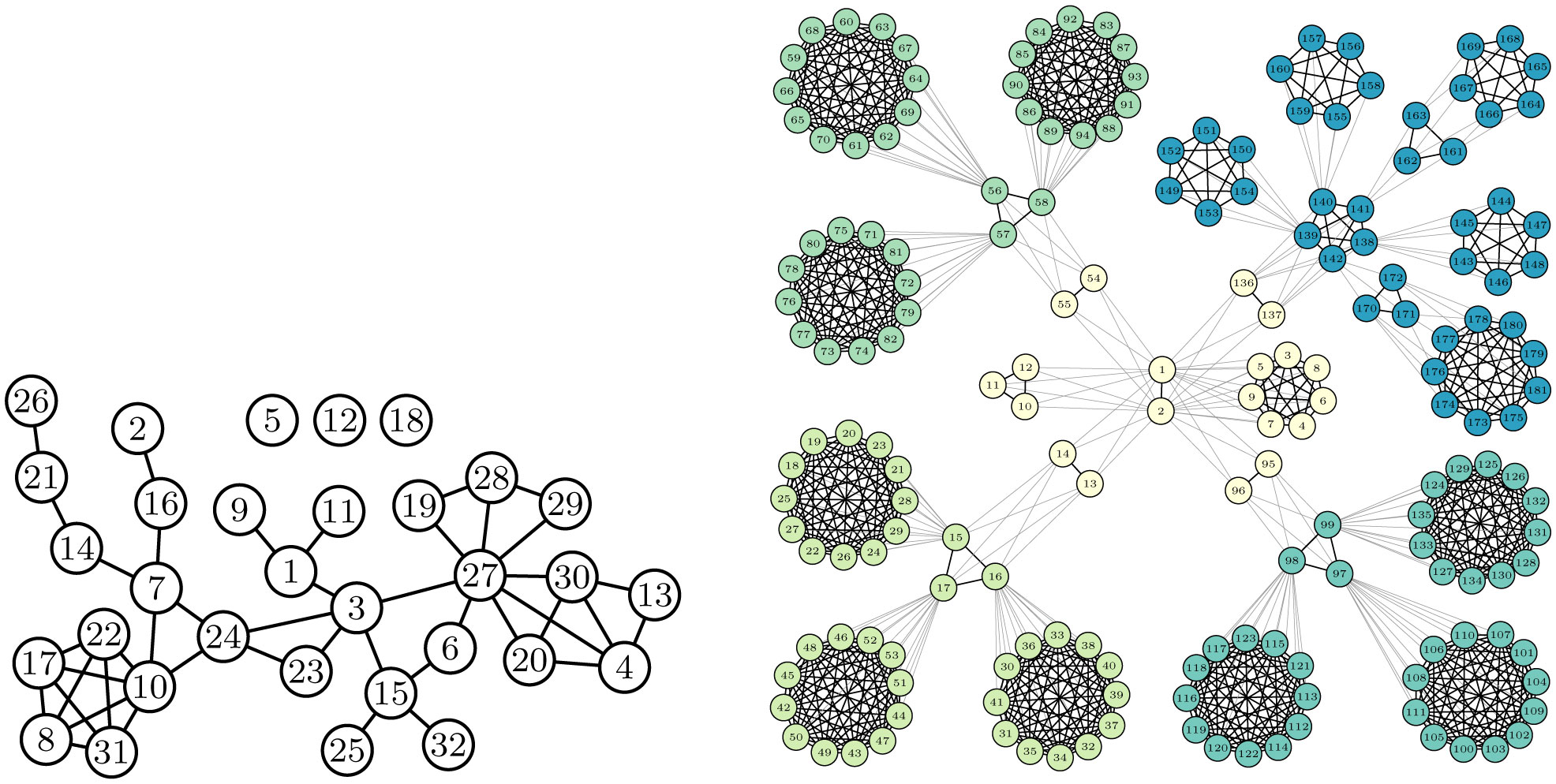
The modelling of epidemic spreading is essential in understanding the mechanisms of outbreaks and pandemics. Many models for different kinds of spreading have been proposed throughout the history of modelling, each suited for a specific scenario and parameters. On the other hand, models of information networks provide important tools for the analysis of the performance and reliability of such networks. We have previously presented a model for simulating the spreading of infectious disease throughout a social network and another one for simulating the connectivity of data traffic in an information network. We argue that these models are similar in that they produce equivalent results with appropriate parameters when run on the same network. We explain this by reasoning that the manners in which the models carry out their calculations, although devised from different assumptions, turn out to be equivalent. We also show empirical results of applying the models to calculate the spread of contagion and information connectivity on two complex networks suitable for the models. Based on the results, we calculate centrality metrics reflecting the outcome of the application, highlighting its important properties. We note that the centrality values obtained by running the epidemic model and the connectivity model turn out to be mutually equivalent, as predicted by their similar fashions of calculation. As the models were independently developed for their own applications, the equivalence in their calculation can not be explained by the models purposefully built similarly. Thus, not only are the two apparently completely separate areas of interest analysable with a single model but there appear to be inherent similarities in the mechanisms of epidemic spreading and determining network connectivity.
- epidemic spreading,
- complex networks,
- immunisation,
- connectivity,
- modelling,
- simulation
Citation: Into Almiala, Vesa Kuikka. Similarity of epidemic spreading and information network connectivity mechanisms demonstrated by analysis of two probabilistic models[J]. AIMS Biophysics, 2023, 10(2): 173-183. doi: 10.3934/biophy.2023011

Related Papers:

Abstract

The modelling of epidemic spreading is essential in understanding the mechanisms of outbreaks and pandemics. Many models for different kinds of spreading have been proposed throughout the history of modelling, each suited for a specific scenario and parameters. On the other hand, models of information networks provide important tools for the analysis of the performance and reliability of such networks. We have previously presented a model for simulating the spreading of infectious disease throughout a social network and another one for simulating the connectivity of data traffic in an information network. We argue that these models are similar in that they produce equivalent results with appropriate parameters when run on the same network. We explain this by reasoning that the manners in which the models carry out their calculations, although devised from different assumptions, turn out to be equivalent. We also show empirical results of applying the models to calculate the spread of contagion and information connectivity on two complex networks suitable for the models. Based on the results, we calculate centrality metrics reflecting the outcome of the application, highlighting its important properties. We note that the centrality values obtained by running the epidemic model and the connectivity model turn out to be mutually equivalent, as predicted by their similar fashions of calculation. As the models were independently developed for their own applications, the equivalence in their calculation can not be explained by the models purposefully built similarly. Thus, not only are the two apparently completely separate areas of interest analysable with a single model but there appear to be inherent similarities in the mechanisms of epidemic spreading and determining network connectivity.

Conflict of interest

All authors declare no conflicts of interest.

References

[1]	(2005) National Research CouncilNetwork Science. Washington: The National Academies Press. https://doi.org/10.17226/11516
[2]	Hu B, Guo H, Zhou P, et al. (2021) Characteristics of SARS-CoV-2 and COVID-19. Nat Rev Microbiol 19: 141-154. https://doi.org/10.1038/s41579-020-00459-7
[3]	Pastor-Satorras R, Castellano C, van Mieghem P, et al. (2015) Epidemic processes in complex networks. Rev Mod Phys 87: 925-979. https://doi.org/10.1103/RevModPhys.87.925
[4]	Valdez LD, Braunstein LA, Havlin S (2020) Epidemic spreading on modular networks: the fear to declare a pandemic. Phys Rev E 101: 032309. https://doi.org/10.1103/PhysRevE.101.032309
[5]	de Arruda GF, Rodrigues FA, Moreno Y (2018) Fundamentals of spreading processes in single and multilayer complex networks. Phys Rep 756: 1-59. https://doi.org/10.1016/j.physrep.2018.06.007
[6]	Nowzari C, Preciado VM, Pappas GJ (2016) Analysis and control of epidemics: a survey of spreading processes on complex networks. IEEE Contr Syst Mag 36: 26-46. https://doi.org/10.1109/MCS.2015.2495000
[7]	Arenas Alex, Cota W, Gómez-Gardeñes J, et al. (2020) Derivation of the effective reproduction number ℛ for COVID-19 in relation to mobility restrictions and confinement. medRxiv . https://doi.org/10.1101/2020.04.06.20054320
[8]	Matamalas JT, Arenas A, Gómez S (2018) Effective approach to epidemic containment using link equations in complex networks. Sci Adv 4: eaau4212. https://doi.org/10.1126/sciadv.aau4212
[9]	Kuikka V (2022) Modelling epidemic spreading in structured organisations. Physica A 592: 126875. https://doi.org/10.1016/j.physa.2022.126875
[10]	Kuikka V, Pham MAA (2022) Models of influence spreading on social networks. Complex Networks & Their Applications X. Cham: Springer International Publishing 112-123. https://doi.org/10.1007/978-3-030-93413-2_10
[11]	Kuikka V, Syrjänen M (2019) Modelling utility of networked services in military environments. In: 2019 International Conference on Military Communications and Information Systems (ICMCIS) . https://doi.org/10.1109/ICMCIS.2019.8842757
[12]	Ball MO, Colbourn CJ, Rovan JS (1995) Chapter 11 Network Reliability. Handbooks in Operations Research and Management Science.Elsevier 673-762. https://doi.org/10.1016/S0927-0507(05)80128-8
[13]	Interdonato R, Atzmueller M, Gaito S, et al. (2019) Feature-rich networks: going beyond complex network topologies. Appl Netw Sci 2019: 4. https://doi.org/10.1007/s41109-019-0111-x
[14]	Amanna IJ, Carlson NE, Slifka MK (2007) Duration of humoral immunity to common viral and vaccine antigens. New Engl J Med 357: 1903-1915. https://doi.org/10.1056/NEJMoa066092
[15]	van de Bunt GG (1999) Friends by choice. An actor-oriented statistical network model for friendship networks through time. University of Groningen, Thela Thesis .
[16]	Delamater PL, Street EJ, Leslie TF, et al. (2019) Complexity of the basic reproduction number (R₀). Emerg Infect Dis 25: 1-4. https://doi.org/10.3201/eid2501.171901

Reader Comments

Your name:*

Email:*
© 2023 the Author(s), licensee AIMS Press. This is an open access article distributed under the terms of the Creative Commons Attribution License (http://creativecommons.org/licenses/by/4.0)