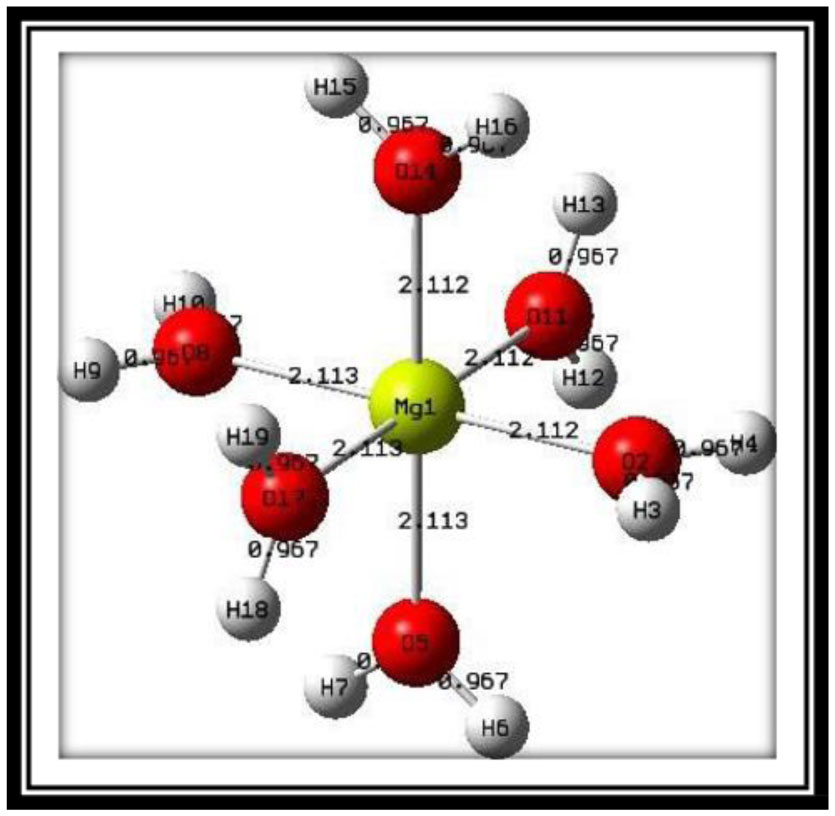
The metal ion is ubiquitous in the human body and is essential to biochemical reactions. The study of the metal ion complexes and their charge transfer nature will be fruitful for drug design and may be beneficial for the extension of the field. In this regard, investigations into charge transport properties from ligands to metal ion complexes and their stability are crucial in the medical field. In this work, the DFT technique has been applied to analyze the delocalization of electrons from the water ligands to a core metal ion. At the B3LYP level of approximation, natural bond orbital (NBO) analysis was performed for the first five distinct complexes [Mg(H2O)6]2+ and [[Mg(H2O)6](H2O)n]2+; n = 1-4. All these complexes were optimized and examined with the higher basis set 6-311++G(d, p). In the complex [Mg(H2O)6]2+, the amount of natural charge transport from ligands towards the metal ion was 0.179e, and the greatest stabilization energy was observed to be 22.67 kcal/mol. The donation of the p orbitals in the hybrid orbitals was increased while approaching the oxygen atoms of H2O ligands in the 1st coordination sphere with the magnesium ions. The presence of water ligands within the 2nd coordination sphere increased natural charge transfer and decreased the stabilizing energy of the complexes. This may be due to the ligand-metal interactions.
Citation: Ganesh Prasad Tiwari, Santosh Adhikari, Hari Prasad Lamichhane, Dinesh Kumar Chaudhary. Natural bond orbital analysis of dication magnesium complexes [Mg(H2O)6]2+ and [[Mg(H2O)6](H2O)n]2+; n=1-4[J]. AIMS Biophysics, 2023, 10(1): 121-131. doi: 10.3934/biophy.2023009
The metal ion is ubiquitous in the human body and is essential to biochemical reactions. The study of the metal ion complexes and their charge transfer nature will be fruitful for drug design and may be beneficial for the extension of the field. In this regard, investigations into charge transport properties from ligands to metal ion complexes and their stability are crucial in the medical field. In this work, the DFT technique has been applied to analyze the delocalization of electrons from the water ligands to a core metal ion. At the B3LYP level of approximation, natural bond orbital (NBO) analysis was performed for the first five distinct complexes [Mg(H2O)6]2+ and [[Mg(H2O)6](H2O)n]2+; n = 1-4. All these complexes were optimized and examined with the higher basis set 6-311++G(d, p). In the complex [Mg(H2O)6]2+, the amount of natural charge transport from ligands towards the metal ion was 0.179e, and the greatest stabilization energy was observed to be 22.67 kcal/mol. The donation of the p orbitals in the hybrid orbitals was increased while approaching the oxygen atoms of H2O ligands in the 1st coordination sphere with the magnesium ions. The presence of water ligands within the 2nd coordination sphere increased natural charge transfer and decreased the stabilizing energy of the complexes. This may be due to the ligand-metal interactions.

| [1] |
Chiu TK, Dickerson RE (2000) 1 Å crystal structures of B-DNA reveal sequence-specific binding and groove-specific bending of DNA by magnesium and calcium. J Mol Biol 301: 915-945. https://doi.org/10.1006/jmbi.2000.4012 
|
| [2] |
Serra MJ, Baird JD, Dale T, et al. (2002) Effects of magnesium ions on the stabilization of RNA oligomers of defined structures. RNA 8: 307-323. https://doi.org/10.1017/S1355838202024226
|
| [3] |
Misra VK, Draper DE (1998) On the role of magnesium ions in RNA stability. Biopolymers: Ori Res Biomol 48: 113-135. https://doi.org/10.1002/(SICI)1097-0282(1998)48:2<113::AID-BIP3>3.0.CO;2-Y
|
| [4] |
Lindahl T, Adams A, Fresco JR (1966) Renaturation of transfer ribonucleic acids through site binding of magnesium. P Natl A Sci 55: 941-948. https://doi.org/10.1073/pnas.55.4.941
|
| [5] |
Mills BJ, Lindeman RD, Lang CA (1986) Magnesium deficiency inhibits biosynthesis of blood glutathione and tumor growth in the rat. P Soc Exp Biol Med 181: 326-332. https://doi.org/10.3181/00379727-181-42260
|
| [6] |
Alfrey AC, Miller NL, Trow R (1974) Effect of age and magnesium depletion on bone magnesium pools in rats. J Clin Invest 54: 1074-1081. https://www.jci.org/articles/view/107851
|
| [7] |
Rude RK, Gruber HE (2004) Magnesium deficiency and osteoporosis: animal and human observations. J Nutr Biochem 15: 710-716. https://doi.org/10.1016/j.jnutbio.2004.08.001
|
| [8] |
Rude RK, Gruber HE, Norton HJ, et al. (2004) Bone loss induced by dietary magnesium reduction to 10% of the nutrient requirement in rats is associated with increased release of substance P and tumor necrosis factor-α. J Nutr 134: 79-85. https://doi.org/10.1093/jn/134.1.79
|
| [9] |
Mohammed HS, Tripathi VD (2020) Medicinal applications of coordination complexes. J Phys: Conf Ser 1664: 012070. https://doi.org/10.1088/1742-6596/1664/1/012070
|
| [10] |
Baaij JHD, Hoenderop JG, Bindels RJ (2015) Magnesium in man: implications for health and disease. Physiol Rev 95: 1-46. https://journals.physiology.org/doi/full/10.1152/physrev.00012.2014
|
| [11] |
Schwalfenberg GK, Genuis SJ (2017) The importance of magnesium in clinical healthcare. Scientifica 2017: 4179326. https://doi.org/10.1155/2017/4179326
|
| [12] |
Sreedhara A, Cowan JA (2002) Structural and catalytic roles for divalent magnesium in nucleic acid biochemistry. Biometals 15: 211-223. https://doi.org/10.1023/A:1016070614042
|
| [13] |
Rijal R, Lamichhane HP, Pudasainee K (2022) Molecular structure, homo-lumo analysis and vibrational spectroscopy of the cancer healing pro-drug temozolomide based on dft calculations. AIMS Biophys 9: 208-220. https://doi.org/10.3934/biophy.2022018
|
| [14] |
Bock CW, Kaufman A, Glusker JP (1994) Coordination of water to magnesium cations. Inorg Chem 33: 419-427. https://doi.org/10.1021/ic00081a007
|
| [15] |
Glendening ED, Feller D (1996) Dication− Water interactions: M2+(H2O)n clusters for alkaline earth metals M= Mg, Ca, Sr, Ba, and Ra. J Phys Chem 100: 4790-4797. https://doi.org/10.1021/jp952546r
|
| [16] |
Rodriguez-Cruz SE, Jockusch RA, Williams ER (1999) Hydration energies and structures of alkaline earth metal ions, M2+(H2O)n, n= 5−7, M= Mg, Ca, Sr, and Ba. J Am Chem Soc 121: 8898-8906. https://doi.org/10.1021/ja9911871
|
| [17] |
Pavlov M, Siegbahn PE, Sandström M (1998) Hydration of beryllium, magnesium, calcium, and zinc ions using density functional theory. J Phys Chem A 102: 219-228. https://doi.org/10.1021/jp972072r
|
| [18] |
Bruzzi E, Raggi G, Parajuli R, et al. (2014) Experimental binding energies for the metal complexes [Mg(NH3)n]2+, [Ca(NH3)n]2+, and [Sr(NH3)n]2+ for n= 4–20 determined from kinetic energy release measurements. J Phys Chem A 118: 8525-8532. https://doi.org/10.1021/jp5022642
|
| [19] |
James C, Raj AA, Reghunathan R, et al. (2006) Structural conformation and vibrational spectroscopic studies of 2, 6-bis (p-N, N-dimethyl benzylidene) cyclohexanone using density functional theory. J Raman Spectrosc 37: 1381-1392. https://doi.org/10.1002/jrs.1554
|
| [20] | Frisch MJ, Trucks GW, Schlegel HB, et al. (2016) Gaussian 16 Revision C. 01. 2016. Wallingford CT: Gaussian Inc. https://gaussian.com/gaussian16/ |
| [21] | Dennington R, Keith TA, Millam JM (2019) Gaussview version 6. semichem Inc.: Shawnee Mission. https://gaussian.com/gaussview6/ |
| [22] |
Becke A (1993) Density-functional thermochemistry.III. The role of exact exchange. J Chem Phys 98: 5648-5652. https://doi.org/10.1063/1.464913
|
| [23] |
Lee C, Yang W, Parr RG (1988) Development of the Colle-Salvetti correlation-energy formula into a functional of the electron density. Phys Rev B 37: 785-789. https://doi.org/10.1103/PhysRevB.37.785
|
| [24] | Yogeswari B, Tamilselvan KS, Thanikaikarasan S, et al. (2022) Quantum density functional theory studies on additive hydration of tuftsin tetrapeptide. J Nanomater . https://doi.org/10.1155/2022/2830708 |
| [25] |
Gangadharan RP, Krishnan SS (2014) Natural bond orbital (NBO) population analysis of 1-azanapthalene-8-ol. Acta Phys Pol A 125: 18-22. http://dx.doi.org/10.12693/APhysPolA.125.18
|
| [26] |
Pokhrel N, Lamichhane HP (2016) Natural bond orbital analysis of [Fe(H2O)6]2+/3+ and [[Zn(H2O)6](H2O)n]2+; n = 0-4. J Phys Chem Biophys 6: 231. http://dx.doi.org/10.4172/2161-0398.1000231
|


Figures(3) / Tables(7)

Ganesh Prasad Tiwari, Santosh Adhikari, Hari Prasad Lamichhane, Dinesh Kumar Chaudhary. Natural bond orbital analysis of dication magnesium complexes [Mg(H2O)6]2+ and [[Mg(H2O)6](H2O)n]2+; n=1-4[J]. AIMS Biophysics, 2023, 10(1): 121-131. doi: 10.3934/biophy.2023009


 DownLoad: