There is increasing interest in the use of DNA polymerases (DNA pols) in next-generation sequencing strategies. These methodologies typically rely on members of the A and B family of DNA polymerases that are classified as high-fidelity DNA polymerases. These enzymes possess the ability to selectively incorporate the correct nucleotide opposite a templating base with an error frequency of only 1 in 106 insertion events. How they achieve this remarkable fidelity has been the subject of numerous investigations, yet the mechanism by which these enzymes achieve this level of accuracy remains elusive. Several smFRET assays were designed to monitor the conformational changes associated with the nucleotide selection mechanism(s) employed by DNA pols. smFRET has also been used to monitor the movement of DNA pols along a DNA substrate as well as to observe the formation of proof-reading complexes. One member among this class of enzymes, the large fragment of Bacillus stearothermophilus DNA polymerase I (Bst pol I LF), contains both 5'→3' polymerase and 3'→5' exonuclease domains, but reportedly lacks exonuclease activity. We have designed a smFRET assay showing that Bst pol I LF forms proofreading complexes. The formation of proofreading complexes at the single molecule level is strongly influenced by the presence of the 3' hydroxyl at the primer-terminus of the DNA substrate. Our assays also identify an additional state, observed in the presence of a mismatched primer-template terminus, that may be involved in the transfer of the primer-terminus from the polymerase to the exonuclease active site.
1.
Introduction
In December 2019, COVID-19 (Corona Virus Disease 2019) named by the World Health Organization was first diagnosed in China. Until now, the COVID-19 in China is basically under control, but there are still many infections around the world. WHO Director-General Tedros Adhanom Ghebreyesus said on March 11, 2020 that COVID-19 has pandemic characteristics. The disease has now spread globally, including cases confirmed in 220 Countries. According to the latest real-time statistics of the WHO, as of November 26, 2020, there have been a total of 60,074,174 confirmed cases of COVID-19, and a total of 1,416,292 deaths [1]. The most infected countries distributed in descending order of infected cases are United States of America, India, Brazil, Russian Federation, France, Spain, The United Kingdom, Italy, etc. To defeat the epidemic, scientists in different fields have contributed to COVID-19 [2,3,4,5,6,7,8,9].
The disease dynamic models continue to play an important role in predicting the development trend of infectious disease epidemics, scientific prevention and control guidance, and provide important data basis and theoretical support for the decision-making of public health managers and the implementation of efficient intervention measures. The SIR model proposed by Kermack and McKendrick [10] has been widely used to study infectious diseases. Differential equations and dynamical system methods are widely used to study the origin, evolution and spread of various diseases. In particular, the dynamic model has achieved fruitful results in rabies [11,12], malaria [13], cholera [14], brucellosis [15] and HFMD(Hand, foot and mouth disease) [16]. There also has been a large amount of literatures using dynamic models to analyze the spread and outbreak of COVID-19 [2,3,8,17,18,19,20,21,22,23,24]. Jiao et al. [2] studied an SEIR with infectivity in incubation period and homestead-isolation on the susceptible. Their research results indicate that governments should strictly implement the isolation system to make every effort to curb the spread of disease during the epidemic. Li et al. [3] revealed the effects of city lock-down date on the final scale of cases and analyzed the impact of the city lock-down date on the final scale of cases by studied the transmission of COVID-19 in Shanxi Province. He et al. [8] proposed an SEIR model for the COVID-19 which is built according to some related factors, such as hospital, quarantine and external input. The particle swarm optimization (PSO) algorithm is applied to estimate the parameters of the system. They show that, for the given parameters, if there exists seasonality and stochastic infection, the system can generate chaos. Bouchnita [17] et al use a multi-scale model of COVID-19 transmission dynamics to quantify the effects of restricting population movement and wearing face masks on disease spread in Morocco. Bardina [19] and Zhang et al. [20] using a stochastic infectious disease model to study COVID-19. This research has shown that the social blockade is very effective in controlling the spread of disease.
For COVID-19, there is no specific vaccines or antiviral drugs to treatment the disease and it is hard to control the spread of the disease. The best way to control the spread of COVID-19 is social blockade. However, the social blockade will have a serious impact on economic development and the normal lives of the people. Therefore, in order not to affect the normal life of non-infected persons, we proposed the strategy of isolating infected people to study the spread of the disease. Nowadays, there is a kind of infectious patients who have no symptoms, disseminating the infection disease and causing social panic. In 2013, Ma et al. [16] established an SEII$ { _\rm a} $HR epidemic model to study the spread of HFMD. The SEII$ { _\rm a} $HR isolates the infected person for treatment, while considering the role of recessive infection in the spread of HFMD. This is the same as our strategy in studying the spread of COVID-19. Therefore, we use the SEII$ { _\rm a} $HR model to study the impact of asymptomatic patients on the disease.
This paper is organized as follows: in the next section, we give the SEII$ { _\rm a} $HR model and describe the each symbol of the system. In section 3, we study the stability analysis of disease-free equilibrium and the persistence of the endemic equilibrium. Next, we take some numerical simulations for the system of (2.1) in section 4. Finally, we give some conclusions about COVID-19.
2.
Mathematical model
From the above discussions, we consider an SEII$ { _\rm a} $HR model with asymptomatic infected and quarantined on the symptomatic infected as following system
Here $ S(t), E(t), I(t), I_{a}(t), H(t), R(t) $ represent the numbers of the susceptible, exposed, symptomatic infected, asymptomatic infected, quarantined, recovered population at time $ t $, respectively. $ \Lambda > 0 $ describes the annual birth rate, $ \beta_{1}, \beta_{2} $ are infection rates, $ \frac{1}{\sigma} $ represents the mean incubation period; $ p $ is the fraction of developing infectious cases, and the remaining fraction $ 1-p $ return to the recessive class; $ \delta_{1} $ and $ \delta_{2} $ are the disease-induced mortality for the infective and quarantined individuals, respectively; $ k $ is the quarantine rate; infective, quarantined and recessive individuals recover at the rate $ \gamma_{1} $, $ \gamma_{2} $ and $ \gamma_{3} $, respectively; $ d $ is the human natural mortality rate.
3.
Stability analysis
Define $ N(t) = S(t)+E(t)+I(t)+I_a(t)+H(t)+R(t) $, from system (2.1), we know that
it implies that the solutions of system (2.1) are bounded and the region
is positively invariant for system (2.1). It is easy to see that system (2.1) has a disease-free equilibrium $ E_0 = (\tfrac{\Lambda}{d}, 0, 0, 0, 0, 0) $. Using the next generation matrix formulated in Diekmam et al. [25] and van den Driessche and Watmough [26], we define the basic reproduction number by
here we denote $ M_1 = \sigma+d, M_2 = \gamma_1+k+\delta_1+d, M_3 = \gamma_3+d $ and $ M_4 = \gamma_2+\delta_2+d $. Thus we have the following theorem.
Theorem 3.1. If $ R_0 < 1 $, then the disease-free equilibrium $ E_0 = (\tfrac{\Lambda}{d}, 0, 0, 0, 0) $ of the system (2.1) is global asymptotically stable.
Proof. we prove the global stability of the disease-free equilibrium. Define the Lypunov function as $ V(E, I, I_a) = \beta_1M_1M_3I+\beta_{2}M_1M_2I_a+\big(\beta_1 \sigma pM_3+\beta_{2}\sigma (1-p)M_2 \big)E $. For all $ t > 0 $, the derivative of $ V(t) $ is
Here the relation $ S\leq \tfrac{\Lambda}{d} $ has been utilized. If $ R_0 < 1 $, we know that $ \tfrac{d V}{dt}\leq 0 $, and $ \tfrac{d V}{dt} = 0 $ holds if and only if $ S = \tfrac{\Lambda}{d} $, $ I = I_a = H = R = 0 $. Using the LaSalle's extension to Lyapunov's method, the limit set of each solution is contained in the largest invariant set in $ \{(S, E, I, I_{a}, H, R)\in X|\tfrac{d V}{dt} = 0\} $ is the singleton $ \{E_0\} $. This means that the disease-free equilibrium $ E_0 $ is globally asymptotically stable in $ X $ when $ R_0 < 1 $.
Theorem 3.2. If $ R_0 > 1 $, then the disease is uniformly persistent, i.e., there is a constant $ \varepsilon > 0 $ such that every positive solution of system (2.1) satisfies
Proof. Define
In order to prove that the disease is uniformly persistent, we only need to show that $ \partial X $ repels uniformly the solutions of system (2.1) in $ X_0 $. It is easy to verify that $ \partial X $ is relatively closed in $ X $ and is point dissipative. Let
We now show that $ X_{\partial} = \{(S_1, 0, 0, 0, 0, 0): 0 < S_1 \leq \tfrac{\Lambda}{d} \} $. Assume that $ x(t)\in X_{\partial} $ for all $ t\geq 0 $, then we have $ E(t) = 0 $ for all $ t\geq0 $. Thus, by the second equation of system (2.1), we have $ S(t)[\beta_{1}I_{1}(t)+\beta_{2}I_{a}(t)] = 0 $, which implies that $ I(t) = 0, I_a(t) = 0 $ for all $ t\geq 0 $. Indeed, if $ I(t)\neq 0, I_a(t)\neq 0 $, there is a $ t_0\geq 0 $ such that $ I(t_0) > 0, I_a(t) > 0 $, form the second equation of system (2.1), we have
It exists a $ t_1 > t_0 $ such that $ E(t_1) > 0, \tfrac{dI}{dt}\big{|}_{t_1} = \sigma p E(t_1) > 0, \tfrac{dI_a}{dt}\big{|}_{t_1} = \sigma (1-p) E(t_1) > 0 $, it follows that there is a $ \eta > 0 $ such that $ I(t), I_a(t) > 0 $ for $ t_1 < t < t_1+\eta $. This means that $ x(t)\notin X_{\partial} $ for $ t_1 < t < t_1+\eta $, which contradicts to the assume $ x(t)\in X_{\partial} $ for all $ t \geq 0 $. Therefore, $ X_{\partial} = \{(S_1, 0, 0, 0, 0, 0): 0 < S_1 \leq \tfrac{\Lambda}{d} \} $.
By analyzing system (2.1), it is clear that $ E_0 $ is unique equilibrium in $ \partial_X $. Next, we will show that $ E_0 $ repels the solutions of system (2.1) in $ X_0 $. We analyze the behavior of any solution $ x(t) $ of system (2.1) close to $ E_0 $. We divide the initial data into two cases.
● If $ E(0) = I(0) = I_a(0) = 0 $, then $ E(t) = I(t) = I_a(t) = 0 $. System (2.1) implies that $ S(t) $ goes away from $ E_0 $ as $ t\rightarrow -\infty $.
● If $ E(0), I(0), I_a(0) > 0 $, then $ E(t), I(t), I_a(t)\geq0 $ for all $ t > 0 $. When $ x(t) $ stays close to $ E_0 $, by the system (2.1) there exists a $ \rho $ small enough such that
where $ \tilde{a}_{11} = -(d+\sigma)-\rho $, $ \tilde{{a}}_{12} = \frac{\Lambda\beta_1}{d}-\rho $, $ \tilde{{a}}_{13} = \frac{\Lambda\beta_2}{d}-\rho $, $ \tilde{a}_{21} = \sigma p $, $ \tilde{a}_{22} = -M_2 $, $ \tilde{a}_{31} = \sigma_1(1-p), \; \tilde{a}_{33} = -(d+\gamma_3), $ and largest eigenvalue of the coefficient matrix $ \tilde{A}(\tilde{a}_{ij}) $ of the right hand of (3.7) is positive, since $ R_0 > 1 $ [25]. Hence the solutions of the linear quasi-monotonic system
with $ y_1(0), y_a(0) > 0 $ are increasing as $ t\rightarrow \infty $. By the comparison principle, $ (E, I_1, I_a) $ goes away from $ (0, 0, 0, 0, 0) $. Therefore, $ \{E_0\} $ is an isolated invariant set and acyclic. Using Theorem 4.3 in Freedman [27], system (2.1) is uniformly persistent. Thus, the proof of Theorem 3.2 is completed.
Biologically speaking, Theorem 3.2 shows that the disease is uniformly persistent if $ R_0 > 1 $, and all the solutions of system are ultimately bounded in $ X $, then system has at least one positive solution By Zhao [28]. Therefore, we have the following theorem.
Theorem 3.3. If $ R_0 > 1 $, then the system (2.1) has an endemic equilibrium $ E_{\star} = (S^{*}, E^{*}, \; I^{*}, I_a^{*}, H^{*}, R^{*}) $.
Proof. From the third and forth equations of system (2.1), we can conclude that
then we have
We also obtain
where $ M_1, M_2, M_3 $ and $ M_4 $ are mentioned in (3.2). Substituting $ S^* $, $ I^* $ and $ I_a^* $ in the second equation of (2.1) at steady state, we obtain the following equation
Here we should show the term $ S^* $ is positive, from the above Eq (3.8), we have $ S^* = \tfrac{M_1M_2M_3}{\beta_1M_3\sigma p+\beta_2M_2\sigma(1-p)} > 0 $. From the similar argument, we have $ I^{*}, I^{*}_{a}, H^*, R^* > 0 $, i.e., the system has at most one positive solution. Therefore, if $ R_0 > 1 $, the system has an endemic equilibrium.
4.
Simulations and results
Since the first case was reported to WHO on 31st December 2019, the COVID-19 has spread rapidly worldwide. As of December 21, 2020 there are 220 countries were infected, and there are many countries still trap in the epidemic. In this section, we consider the study of spread of COVID-19 disease in India. India is observing an increase in the number of patients each day. The accuracy of our proposed model is validated by using the official data of India from[29,30,31].
The study consider currently infected patients of India from May 1st 2020 to November 15th 2020. The population of India is around $ N = 1386750000 $[29], thus we assumed that the initial value is $ S(0) = N-E(0)-I_{a}(0)-I(0)-H(0)-R(0) $, $ E(0) = 315236 $, $ I_{a} = 78809 $, $ I(0) = 236427 $, $ H(0) = 7880 $, $ R(0) = 59646 $. Then we illustrate the source of parameters in following. We can get the value of population input into the susceptible class through birth 77575 per day in India, and the average life expectancy of India is 70.42. Noting that $ 1/d $ is the average life expectancy, the value of parameter $ d $ can be calculated as $ d = 1/(70.42\times365) = 3.8904\times10^{-5} $. We choose the $ 1/\sigma = 2.5 $ which represent the average period of from the susceptible to the exposed. Because the average recovered period of the quarantined about is 14 days, so we choose the parameter $ \gamma_{2} = 1/14 = 0.0714 $. The parameters of system (2.1) are listed in Table 1.
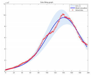
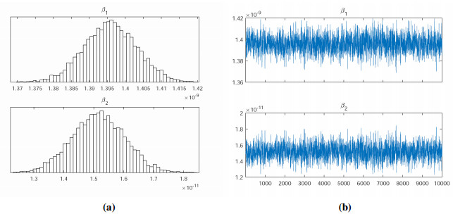
We use the Markov Chain Monte Carlo (MCMC) method to fit the parameters $ \beta_{1} $, $ \beta_{2} $ to the data, and adopt an adaptive Metropolis-Hastings (M-H) algorithm to carry out the MCMC procedure. The algorithm is run for 10,000 iterations with a burn-in of the first 6,000 iterations, and the Geweke convergence diagnostic method is employed to assess convergence of chains. In Figure 1, we have plotted the curves between the total number of COVID-19 cases versus days (till November 15, 2020) in India based on the actual data and the proposed model (2.1). The estimation results some parameters are given in Table 2 and Figure 2.
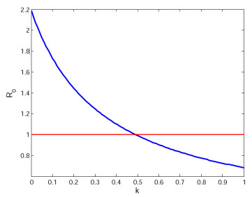
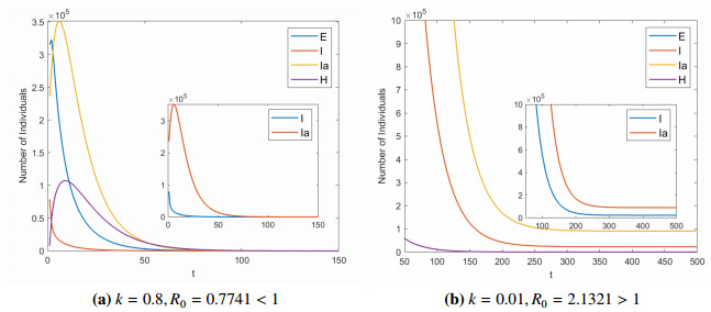
For the quarantine rate $ k $, we have chosen two different values as a comparison to show the importance of quarantine measures for symptomatic infected to control the spread of disease. Figure 3 shows the relationship between quarantine rate $ k $ and basic reproduction number $ R_{0} $. We can see that $ R_{0} $ and $ k $ are negatively correlated. After calculation, we get the critical point $ k_{c} = 0.4949 $, then we have $ R_{0} $ is equal to 1. Figure 4 is the evolution of system (2.1) when $ k = 0.8 $, $ 0.01 $, respectively. If $ k = 0.8 $, we compute the basic reproduction number $ R_{0} = 0.7741 < 1 $, it can be seen that the disease-free equilibrium $ E_{0} $ is globally asymptotically stable (see Figure 4a). If $ k = 0.01 $, we calculate the basic reproduction number $ R_{0} = 2.1321 > 1 $, it can be seen that system (2.1) has a positive equilibrium point and it is is uniformly persistent (see Figure 4b).
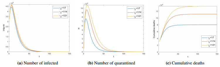
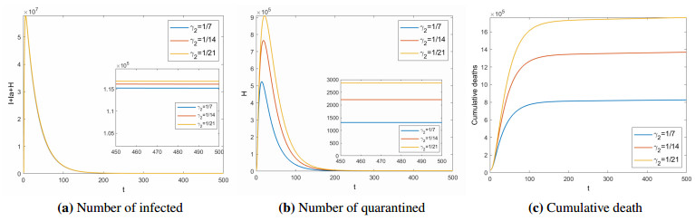
Next, the impact of the treatment period($ 1/\gamma_{2} $) for quarantined on COVID-19 is analyzed. Figures 5 and 6 show the number of infected ($ I+I_{a}+H $), quarantined ($ H $), and cumulative deaths (COVID-19 deaths, excluding natural deaths) in different treatment period for $ R_{0} < 1 $ and $ R_{0} > 1 $ respectively. When $ R_{0} < 1 $, the shorter the treatment period, the disease will die out faster, and the fewer people will be isolated. At the same time, the cumulative number of deaths will be lower. When $ R_{0} > 1 $, the longer the treatment period, the more people will be infected and quarantined. Assuming that there are no individual differences, the treatment period is negatively related to the medical level. That is, the higher the medical level, the shorter the treatment period. This means that improving the level of medical treatment is conductive to the control of COVID-19. Therefore, it is urgent for India and other countries to develop specific drugs against COVID-19.
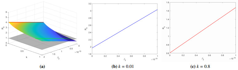
Then, we show the relationship between parameters $ k, \beta_2 $ and $ R_0 $. From Figure 7a, we know that the parameters $ k $ and $ R_{0} $ are negatively correlated, and the parameters $ \beta_2 $ and $ R_{0} $ are positively correlated. When $ \beta_{2} = 2.0\times10^{-11} $, the quarantine rate $ k $ has the maximum threshold $ k = 0.5411 > k_{c} $. When $ \beta_2 = 0 $, the quarantine rate $ k $ has the minimum threshold $ k = 0.3519 < k_{c} $. Figure 7b, 7c show the relationship between $ \beta_2 $ and $ R_0 $ when $ k = 0.01, 0.8 $, respectively. When $ k = 0.01 $, the disease is uniformly persistent, even the the parameter $ \beta_2 = 0 $. If we select $ k = 0.8 $, only when $ \beta_2 > 3.6639\times10^{-11} $ can affect the spread of the disease. Therefore, we deduce that when $ k > 0.5411 $, asymptomatic infections do not affect the spread of the disease; when $ 0.3519 < k < 0.5411 $, it is related to the infection rate of asymptomatic people whether the disease persists. In general, the higher the quarantine rate of people with symptoms, the easier it is to control the spread of the disease.
5.
Conclusions
In this paper, we consider an SEII$ { _\rm a} $HR epidemic model with asymptomatic infection and isolation. First, We have proved that the disease-free equilibrium $ E_{0} $ is globally asymptotically stable if and only if $ R_{0} < 1 $ and the system (2.1) is uniformly persistent if $ R_{0} > 1 $. Our numerical simulation results are consistent with theoretical analysis. Second, we showed the impact of the treatment period($ 1/\gamma_{2} $) for quarantined on COVID-19. The better the medical treatment, the COVID-19 is more likely to die out or be controlled at a lower level. Therefore, it is urgent for India and other countries around the world to develop specific drugs against COVID-19. Third, we deduced that the parameters $ k $ and $ R_{0} $ are negatively correlated, and the parameters $ \beta_{2} $ and $ R_{0} $ are positively correlated. At the same time, we found that asymptomatic infections will affect the spread of the disease when the quarantine rate is within the range of $ [0.3519, 0.5411] $ and isolating people with symptoms is very important to control and eliminate the disease in India and other countries.
Acknowledgments
The authors would like to thank the referees for helpful comments which resulted in much improvement of the paper. Project Supported by National Nature Science Foundation of China (Grant No. 12071445, 12001501), Fund for Shanxi 1331KIRT, Shanxi Natural Science Foundation (Grant No. 201901D211216) and the outstanding youth fund of North University of China.
Conflict of interest
The authors declare that they have no conflict of interest.


 DownLoad: