Finite state machine and Markovian equivalents of the <i>lac</i> Operon in <i>E. coli</i> bacterium

Urooj Ainuddin; Maria Waqas; Urooj Ainuddin; Maria Waqas

doi:10.3934/bioeng.2022029

AIMS Bioengineering

2022, Volume 9, Issue 4: 400-419. doi: 10.3934/bioeng.2022029

Previous Article Next Article

Research article

Finite state machine and Markovian equivalents of the lac Operon in E. coli bacterium

Urooj Ainuddin ^,,
Maria Waqas

Department of Computer and Information Systems Engineering, NED University of Engineering and Technology, Karachi, 75270, Pakistan

Received: 10 November 2022 Revised: 07 December 2022 Accepted: 11 December 2022 Published: 28 December 2022

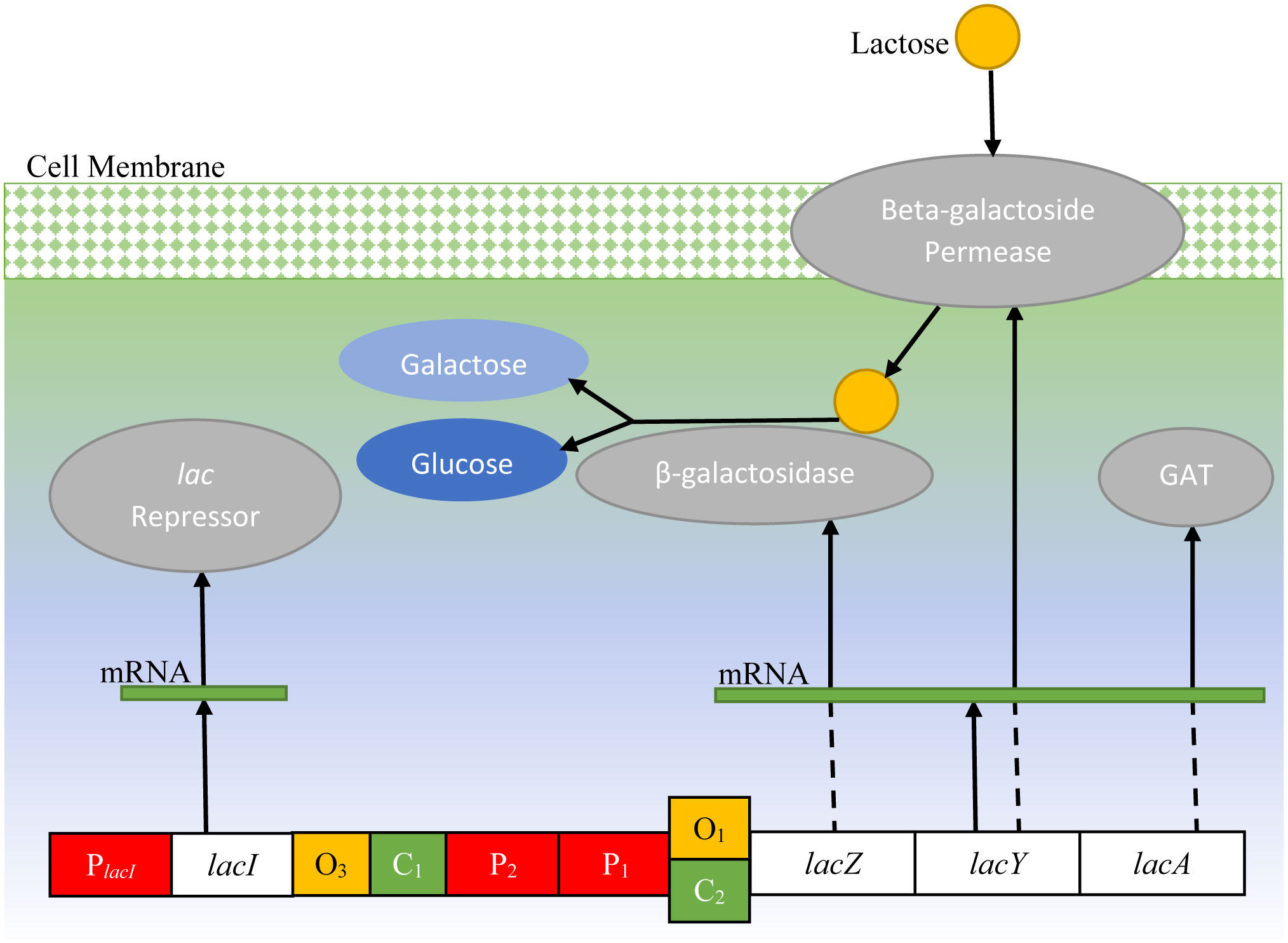
The lac operon in E. coli has been extensively studied by computational biologists. The bacterium uses it to survive in the absence of glucose, utilizing lactose for growth. This paper presents a novel modeling mechanism for the lac operon, transferring the process of lactose metabolism from the cell to a finite state machine (FSM). This FSM is implemented in field-programmable gate array (FPGA) and simulations are run in random conditions. A Markov chain is also proposed for the lac operon, which helps study its behavior in terms of probabilistic variables, validating the finite state machine at the same time. This work is focused towards conversion of biological processes into computing machines.
- digital modeling,
- lac operon,
- bistable switch,
- finite state machine,
- Markov model
Citation: Urooj Ainuddin, Maria Waqas. Finite state machine and Markovian equivalents of the lac Operon in E. coli bacterium[J]. AIMS Bioengineering, 2022, 9(4): 400-419. doi: 10.3934/bioeng.2022029

Related Papers:

Abstract

The lac operon in E. coli has been extensively studied by computational biologists. The bacterium uses it to survive in the absence of glucose, utilizing lactose for growth. This paper presents a novel modeling mechanism for the lac operon, transferring the process of lactose metabolism from the cell to a finite state machine (FSM). This FSM is implemented in field-programmable gate array (FPGA) and simulations are run in random conditions. A Markov chain is also proposed for the lac operon, which helps study its behavior in terms of probabilistic variables, validating the finite state machine at the same time. This work is focused towards conversion of biological processes into computing machines.

Conflict of interest

The Authors declare that there is no conflict of interest.

References

[1]	Ainuddin U, Khurram M, Hasan SMR (2019) Cloning the λ Switch: digital and Markov representations. IEEE Trans NanoBiosci 18: 428-436. https://doi.org/10.1109/TNB.2019.2908669
[2]	Alspector J, Gannett J W, Haber S, et al. (1990) Generating multiple analog noise sources from a single linear feedback shift register with neural network application. ISCAS 1990: 1058-1061.
[3]	Angelova M, Ben-Halim A (2011) Dynamic model of gene regulation for the lac operon. J Phys Conf Ser 286: 012007. https://doi.org/10.1088/1742-6596/286/1/012007
[4]	Balaeff A, Mahadevan L, Schulten K (2004) Structural basis for cooperative DNA binding by CAP and lac repressor. Structure Structure 12: 123-132. https://doi.org/10.1016/j.str.2003.12.004
[5]	Brenguier D, Chaouiya C, Monteiro P T, et al. (2013) Dynamical modeling and analysis of large cellular regulatory networks. Chaos 23: 025114. https://doi.org/10.1063/1.4809783
[6]	Berg JM, Tymoczko JL, Stryer L, et al. (2002) Biochemistry. New York: W. H. Freeman.
[7]	Bchel DE, Gronenborn B, Mller-Hill B (1980) Sequence of the lactose permease gene. Nature 283: 541-545. https://doi.org/10.1038/283541a0
[8]	Calder M, Vyshemirsky V, Gilbert D, et al. (2006) Analysis of signalling pathways using continuous time Markov chains. Transactions on Computational Systems Biology VI. Heidelberg: Springer 44-67.
[9]	Chatterjee S, Rothenberg E (2012) Interaction of bacteriophage λ with its E. coli receptor, lamB. Viruses 4: 3162-3178. https://doi.org/10.3390/v4113162
[10]	Choudhary K, Narang A (2019) Analytical expressions and physics for single-cell mRNA distributions of the lac Operon of E. coli. Biophys J 117: 572-586. https://doi.org/10.1016/j.bpj.2019.06.029
[11]	Daber R, Stayrook S, Rosenberg A, et al. (2007) Structural analysis of lac repressor bound to allosteric effectors. J Mol Biol 370: 609-619. https://doi.org/10.1016/j.jmb.2007.04.028
[12]	Donnelly CE, Reznikoff WS (1987) Mutations in the lac P2 promoter. J Bacteriol 169: 1812-1817. https://doi.org/10.1128/jb.169.5.1812-1817.1987
[13]	Eshra A, El-Sayed A (2014) An odd parity checker prototype using DNAzyme finite state machine. IEEE/ACM Trans Comput Biol Bioinform 11: 316-324. https://doi.org/10.1109/TCBB.2013.2295803
[14]	Esmaeili A, Davison T, Wu A, et al. (2015) PROKARYO: an illustrative and interactive computational model of the lactose operon in the bacterium Escherichia coli. BMC Bioinformatics 16: 1-23. https://doi.org/10.1186/s12859-015-0720-z
[15]	Fang X, Liu Q, Bohrer C, et al. (2018) Cell fate potentials and switching kinetics uncovered in a classic bistable genetic switch. Nat Commun 9: 2787. https://doi.org/10.1038/s41467-018-05071-1
[16]	Gao R, Hu W Study on some modeling problems in the process of gene expression with finite state machine (2012)2012: 5066-5070. https://doi.org/10.1109/WCICA.2012.6359438
[17]	Gao R, Hu W, Tarn TJ (2013) The application of finite state machine in modeling and control of gene mutation process. IEEE Trans NanoBiosci 12: 265-274. https://doi.org/10.1109/TNB.2013.2260866
[18]	Gebali F (2008) Analysis of Computer and Communication Networks. US: Springer. https://doi.org/10.1007/978-0-387-74437-7
[19]	Griffiths AJ, Gelbart WM, Miller JH, et al. (1999) Darwin's Revolution. Modern Genetic Analysis. New York: W. H. Freeman.
[20]	Hasan SMR (2010) A digital cmos sequential circuit model for bio-cellular adaptive immune response pathway using phagolysosomic digestion: a digital phagocytosis engine. J Biomed Sci Eng 3: 470-475. https://doi.org/10.4236/jbise.2010.35065
[21]	Jacob C, Burleigh I (2004) Biomolecular swarms–an agent-based model of the lactose operon. Nat Comput 3: 361-376. https://doi.org/10.1007/s11047-004-2638-7
[22]	Jacob F, Monod J (1961) Genetic regulatory mechanisms in the synthesis of proteins. J Mole Biol 3: 318-356. https://doi.org/10.1016/S0022-2836(61)80072-7
[23]	Julius AA, Halasz A, Kumar V, et al. (2006)2006: 19-24. https://doi.org/10.1109/CDC.2006.376739
[24]	Krogh A, Larsson B, Von Heijne G, et al. (2001) Predicting transmembrane protein topology with a hidden Markov model: application to complete genomes. J Mole Biol 305: 567-580. https://doi.org/10.1006/jmbi.2000.4315
[25]	Lawson CL, Swigon D, Murakami KS, et al. (2004) Catabolite activator protein: DNA binding and transcription activation. Curr Opin Struct Biol 14: 10-20. https://doi.org/10.1016/j.sbi.2004.01.012
[26]	Li H, Wang S, Li X, et al. (2020) Perturbation analysis for controllability of logical control networks. SIAM J Control Optim 58: 3632-3657. https://doi.org/10.1137/19M1281332
[27]	Mahaffy JM, Savev ES (1999) Stability analysis for a mathematical model of the lac operon. Quart Appl Math 57: 37-53. https://doi.org/10.1090/qam/1672171
[28]	McAdams HH, Shapiro L (1995) Circuit simulation of genetic networks. Science 269: 650-656. https://doi.org/10.1126/science.762479
[29]	Moore EF (1956) Gedanken-experiments on sequential machines. Automata Studies 34: 129-153. https://doi.org/10.1515/9781400882618-006
[30]	Muri F (1998) Modelling bacterial genomes using hidden Markov models. COMPSTAT 1998: 89-100. https://doi.org/10.1007/978-3-662-01131-7-8
[31]	Vergne N (2008) Drifting Markov models with polynomial drift and applications to DNA sequences. Stat Appl Genet Mol Biol 7: 6. https://doi.org/10.2202/1544-6115.1326
[32]	Notley-McRobb L, Death A, Ferenci T (1997) The relationship between external glucose concentration and cAMP levels inside Escherichia coli: implications for models of phosphotransferase-mediated regulation of adenylate cyclase. Microbiology 143: 1909-1918. https://doi.org/10.1099/00221287-143-6-1909
[33]	Novick A, Weiner M (1957) Enzyme induction as an all-or-none phenomenon. Proc Natl Acad Sci USA 43: 553-566. https://doi.org/10.1073/pnas.43.7.553
[34]	Oehler S, Amouyal M, Kolkhof P, et al. (1994) Quality and position of the three lac operators of E. coli define efficiency of repression. EMBO J 13: 3348-3355. https://doi.org/10.1002/j.1460-2075.1994.tb06637.x
[35]	Oehler S, Eismann ER, Krmer H, et al. (1990) The three operators of the lac operon cooperate in repression. EMBO J 9: 973-979. https://doi.org/10.1002/j.1460-2075.1990.tb08199.x
[36]	Oishi K, Klavins E (2014) Framework for engineering finite state machines in gene regulatory networks. ACS Synth Biol 3: 652-665. https://doi.org/10.1021/sb4001799
[37]	Rani MJ, Malarkkan S (2012) Design and analysis of a linear feedback shift register with reduced leakage power. Int J Comput Appl 56: 9-13. https://doi.org/10.5120/8957-3159
[38]	Hasan SMR (2008) A novel mixed-signal integrated circuit model for DNA-protein regulatory genetic circuits and genetic state machines. IEEE Trans Circuits Syst Regul Pap 55: 1185-1196. https://doi.org/10.1109/TCSI.2008.925632
[39]	Reznikoff WS (1992) Catabolite gene activator protein activation of lac transcription. J Bacteriol 174: 655-658. https://doi.org/10.1128/jb.174.3.655-658.1992
[40]	Ross SM (2010) Introduction to Probability Models. Boston: Academic Press ocn444116127. https://doi.org/10.1016/B978-0-12-375686-2.00007-8
[41]	Saad Y (2011) Numerical methods for large eigenvalue problems: revised edition. USA: SIAM. https://doi.org/10.1137/1.9781611970739
[42]	Santilln M (2008) Bistable behavior in a model of the lac operon in Escherichia coli with variable growth rate. Biophys J 94: 2065-2081. https://doi.org/10.1529/biophysj.107.118026
[43]	Santilln M, Mackey MC (2004) Influence of catabolite repression and inducer exclusion on the bistable behavior of the lac operon. Biophys J 86: 1282-1292. https://doi.org/10.1016/S0006-3495(04)74202-2
[44]	Shenker JQ, Lin MM (2015) Cooperativity leads to temporally-correlated fluctuations in the bacteriophage lambda genetic switch. Front Plant Sci 6: 214. https://doi.org/10.3389/fpls.2015.00214
[45]	Shmulevich I, Dougherty ER, Zhang W (2002) From Boolean to probabilistic Boolean networks as models of genetic regulatory networks. Proc IEEE 90: 1778-1792. https://doi.org/10.1109/JPROC.2002.804686
[46]	Shuman HA, Silhavy TJ (2003) The art and design of genetic screens: Escherichia coli. Nat Rev Genet 4: 419-431. https://doi.org/10.1038/nrg1087
[47]	Suen G, Jacob C (2003) A symbolic and graphical gene regulation model of the lac operon. Challenging the Boundaries of Symbolic Computation. London: Imperial College 73-80. https://doi.org/10.1142/9781848161313-0010
[48]	Floyd TL (2015) Digital Fundamentals. England: Pearson Education.
[49]	Veliz-Cuba A, Stigler B (2011) Boolean models can explain bistability in the lac operon. J Comput Biol 18: 783-794. https://doi.org/10.1089/cmb.2011.0031
[50]	Vossen KM, Stickle DF, Fried MG (1996) The Mechanism of CAP-lacRepressor Binding Cooperativity at the E. coliLactose promoter. J Mol Biol 255: 44-54. https://doi.org/10.1006/jmbi.1996.0005
[51]	Wang S, Zhang Y, Ouyang Q (2006) Stochastic model of coliphage lambda regulatory network. Phys Rev E 73: 041922. https://doi.org/10.1103/PhysRevE.73.041922
[52]	Wong P, Gladney S, Keasling JD (1997) Mathematical model of the lac operon: inducer exclusion, catabolite repression, and diauxic growth on glucose and lactose. Biotechnol Prog 13: 132-143. https://doi.org/10.1021/bp970003o
[53]	Yang J, Meng X, Hlavacek WS (2010) Rule-based modelling and simulation of biochemical systems with molecular finite automata. IET Syst Biol 4: 453-466. https://doi.org/10.1049/iet-syb.2010.0015
[54]	Yildirim N, Kazanci C (2011) Deterministic and stochastic simulation and analysis of biochemical reaction networks: The lactose operon example. Methods in Enzymology. New York: Academic Press 371-395. https://doi.org/10.1016/B978-0-12-381270-4.00012-3
[55]	Yildirim N, Mackey MC (2003) Feedback regulation in the lactose operon: a mathematical modeling study and comparison with experimental data. Biophys J 84: 2841-2851. https://doi.org/10.1016/S0006-3495(03)70013-7
[56]	Yildirim N, Santillan M, Horike D, et al. (2004) Dynamics and bistability in a reduced model of the lac operon. Chaos 14: 279-292. https://doi.org/10.1063/1.1689451

bioeng-09-04-029-s001.pdf

Reader Comments

Your name:*

Email:*
© 2022 the Author(s), licensee AIMS Press. This is an open access article distributed under the terms of the Creative Commons Attribution License (http://creativecommons.org/licenses/by/4.0)