Pomegranates (Punica granatum) are a significant source of bioactive compounds and have been widely used in traditional Eastern medicine in different countries and cultures. Pomegranate peel and pulp have significantly antioxidant capacity, and pomegranate pulp contain markedly anti-atherogenic activity against atherosclerosis diseases in humans and mice model investigations. Pomegranates from different cultivars possess different bioactive molecules, increasing the desired antioxidant properties genes and chemical profiles. This study provides an overview of geographic origins and an evaluation of the chemical analysis of flavonoids and polyphenolic content of the pomegranate from the local (Persian) and foreign pomegranate cultivars. The present narrative review aims to compare chemical analysis of total phenolic and flavonoids content of different pomegranate cultivars grown in various geographic regions in the world. This review demonstrated that remarkable differences existed in all factors rates measured in various cultivars, being considerably related to many factors such as cultivar type, growing region, maturity, cultivation, climate, edaphic condition, and storage situation. The data would be useful to produce better crops with high nutritional quality.
1.
Introduction
Fetal well-being during pregnancy has been widely assessed with fluctuations of fetal heart rate or fetal heart rate variability (FHRV) monitoring. Recently there has been increasing interest in research on maternal-fetal heart rate coupling for assessing fetal heath which would not be evaluated with the traditional temporal and spectral methods applied directly to fetal heart rate recordings [1]. Previous studies have shown variations in FHRV due to physiological and psychological states of the mother such as maternal stress and anxiety, exercise and low level of blood oxygen resulted in FHR changes [2,3,4].
Various signal processing methods were used to study the coupling between mother and fetus [1,4,5,6,7]. For example, Khandoker et al. applied normalized short time partial directed coupling (NSTPDC) to show strong influence of fetal heart rate on maternal heart rate in the early gestation [5]. This influence decreased significantly from early to mid-gestation and was associated with a significant increase of maternal to fetal coupling strength [5]. Van Leeuwen et al. have shown beat by beat synchronization between mother and fetus heartbeats by using phase synchronization [7].
The specific mechanism leading to maternal–fetal heart rate coupling remains unexplained and previous studies [7,8] proposed two hypotheses for pathways mediating this interaction: (ⅰ) the oscillatory rhythm of maternal respiration acts as a common driving force and influences simultaneously both maternal and fetal heart rates, leading to an apparent maternal–fetal heartbeat synchronization; (ⅱ) the maternal cardiac system has a direct acoustic stimulus effect on the fetal heart rhythm.
Recently assessment of the strength's relations and their directionality of couplings have been two major aspects of investigations for a more detailed understanding of physiological regulatory mechanisms [9,10]. There are several approaches used to assess direct and indirect couplings that can be grouped into five classes basing on traditional domain classification as Granger causality, nonlinear prediction, entropy, symbolization and phase synchronization [11,12,13,14,15,16]. For nonlinear interaction analysis between heart rate, blood pressure and/ or respiratory time series the method of Joint Symbolic Dynamics (JSD, [12]) and High Resolution Joint Symbolic Dynamics (HRJSD, [17,18]) were applied. The principle of joint symbolic dynamics is to analyze nonlinear couplings between two time series based on the analysis of bivariate dynamic processes by means of symbols. Symbolization based methods enable a coarse grain quantitative assessment of short-term dynamics of time series for direct analysis of successive signal amplitudes based on discrete states (symbols) [11]. JSD quantifies coupling between two systems using two symbols: 0 and 1. Using JSD, Reulecke et al. have shown some independent heart rate regulation patterns from the respiratory regulation in quiet sleep of preterm neonates which was interpreted as an increase in the vagal modulation [19]. HRJSD was also proposed to quantify short-term cardiovascular couplings in acute schizophrenia [18]. HRJSD uses three symbols 0, 1 and 2 to characterize coupling between two systems. Schultz et al. have applied HRJSD to study baroreflex changes due to medication in a group of schizophrenia patients. They have shown an increase in the invariable BBI-E1 pattern (no variation or unchanged BBI of type 1 symbols) coupled with alternating systolic pressure (SP) families: SP-E2 (unchanged SP in type 2 patterns), SP-LU1 (one variation in three words of SP), SP-P (three variations in SP) in medicated schizophrenia patients compared to unmedicated patients. This was interpreted as impairment of the baroreflex feedback loop (which is parasympathetic) due to the anti-cholinergic effect of the antipsychotics [18].
In our previous study, HRJSD was used to study gestational age effect on healthy maternal-fetus coupling. The observed diminished fluctuating and alternating fetal heart rate patterns and intensified fast and strong fetal heart rate changes from the first to the third trimester could be an indicator of more matured adaptation of autonomic nervous system (ANS) to strong short-term maternal heart rate changes as external stimuli [20].
In this study, HRJSD method was applied to study short-term maternal-fetal cardiac couplings in abnormal cases (diseased mothers) and compare them to the healthy cases (normal pregnancies). The aim was to evaluate whether HRJSD could work as a noninvasive measure for screening fetal cardiac anomalies at an early stage.
2.
Materials and method
2.1. Subjects
Recording of the maternal and abdominal ECG signals (mECG and abECG) from 85 pregnant women at the gestational age of 16~41 weeks were collected from Tohoku University Hospital. Among these cases, 66 were normal single pregnancies and 19 were abnormal pregnancies with different types of abnormality (GAa (19-38 weeks). The normal cases were divided into three gestational age groups: GA1 (16–25 weeks), GA2 (26–30 weeks) and GA3 (32–40 weeks) and each of the groups has 22 subjects. The abnormal group has variety of abnormality such as: bradycardia, tachycardia, premature atrial contraction and different types of congenital heart defects (CHD) or anomalies (ventriculoseptal defect (VSD), atrial septal defect (ASD), pulmonary atresia (PA), tetralogy of Fallot (TOF) and Ebstain anomaly). Tables 1, 2 show demographics of the normal and abnormal cases. The study protocol was approved by Tohoku University Institutional Review Board and written informed consent were obtained from all subjects.
2.2. Data preprocessing
All recordings (each of 1 minute's length) were sampled at 1000 Hz with 16-bit resolution. Fetal ECG (fECG) traces were extracted using a method that combines cancellation of the mother's ECG signal and the blind source separation with reference (BSSR) as described in our earlier study [21]. Intervals between successive R waves of the QRS complex (i.e., R-R intervals in seconds) were calculated using the algorithm developed by Pan and Tompkins [22]. Two beat-to-beat intervals (BBI) time series namely fetal heart rates (fBBI) and maternal heart rates (mBBI) were extracted from R-R intervals of mECG and fECG signals. Both time series were visually inspected and if appropriate reedited. Afterwards these time series (fBBI, mBBI) were subsequently filtered by an adaptive filter algorithm to remove and interpolate ventricular premature beats and artefacts to obtain normal-to-normal beat time series. For the maternal-fetal coupling analyses the filtered fBBI and filtered mBBI time series were resampled (spline interpolation) using frequency fs = 5Hz.
2.3. High resolution joint symbolic dynamics (HRJSD)
HRJSD was developed to analyze nonlinear cardiovascular couplings in acute schizophrenia patients based on the analysis of dynamic processes by using symbols [18]. In this study we used HRJSD for quantifying the fetal-maternal heart rate couplings. Therefore, both time series (fBBI and mBBI) were transformed into symbol sequences. If X is a bivariate signal vector, xnfBBI and xnmBBI respectively.
X is then transformed into a bivariate symbol vector S which defined as
The definitions of symbols are as follows:
similarly
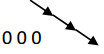
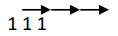
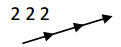
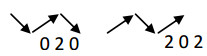
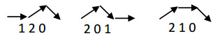
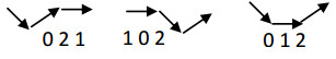
and the threshold levels lfBBI and lmBBI were considered to be 0. Symbol sequences with increasing values were coded as "2", decreasing values were coded as "0" and unchanging (no variability) values were coded as "1". The symbol vector S was subdivided into short words (bin) wk of word length k = 3. Thus, using three symbols led to 27 different word types for fBBI (wfBBI) and mBBI (wmBBI) were formed and total of number of all word type combination were 729 = 27 × 27. Then all single word types wfBBI, mBBI were grouped into 8 pattern families' wf whereby the probabilities of all single word family's occurrences p(wf) was normalized to 1. There were 8 pattern families (E0, E1, E2, LU1, LD1, LA1, P, V) which represent different aspects of autonomic modulation and were sorted into an 8x8 pattern family density matrix Wf resulting in 64 maternal-fetal coupling patterns. The pattern definitions are shown in Table 3 and the effects on the BBI are shown in Table 4. Additionally, the sum of each (n = 8) column cfmBBI, the sum of each (n = 8) row cffBBI and the Shannon entropy (HRJSDshannon) of Wf were calculated from the matrix Wf as a measure of overall complexity of fetal maternal coupling.
2.4. Statistics
In this study the nonparametric Mann-Whitney U-test was performed to check the differences between the normal and abnormal groups. Significances were considered for values of p < 0.05. All results were presented as mean ± SD. Due to their limited numbers, qualitative comparisons were also made between some abnormality types (such as AV block and tachycardia) and the normal fetuses.
3.
Results
3.1. Normal pregnancies
Figure 1 show a 3D bar plot of averaged pattern family density matrix Wf for the three normal groups and some abnormal cases. The coupling patterns between maternal and fetal time series were consistent for all three normal gestational age groups but with different strength. For example, GA1 has higher probability of occurrence; p(wf) for mBBI-E0/fBBI-LD1, mBBI-E0/fBBI-LU1 and mBBI-E2/fBBI-LD1 than GA2 and GA3 (Figure 1a–c). On the other hand, GA2 and GA3 showed higher p(wf) for mBBI-E0/fBBI-E0 and mBBI-E2/fBBI-E0 than GA1 (it was statistically significant for GA3 only). The E1, P and V patterns were completely absent in both mBBI and fBBI time series for GA1, GA2, and GA3. The significant coupling patterns between the three groups was reported in our previous work (Table 5)[20]. No significant differences were found between GA2 and GA3 which indicates that these coupling patterns do not capture changes in the development of the ANS between middle and late gestational weeks. Coupling between fetal E0 and maternal E0, E2 and LD1 patterns was significantly higher in late groups (GA3) compared to GA1, while coupling between fetal LA1 and maternal E0, LU1 and LD1 and between fetal LD1 and maternal E2 and LU1 was significantly lower for late groups (GA3).
3.2. Normal pregnancies vs. abnormal pregnancies
For the abnormal cases (AV block) revealed higher p(wf) for fetal patterns E0 and E2 (fBBI-E0, fBBI-E2), and lower p(wf) for fetal patterns LU1 and LD1 (fBBI-LU1, fBBI-LD1) with mBBI-E0, E2, LU1 and LD1 maternal patterns than all normal groups. The fetal pattern LA1 (fBBI-LA1) diminished with the exception in combination with mBBI-E2 (Figure 1-d).
For the tachycardia case (Figure 1-e), p(wf) for the maternal patterns (mBBI-E0, E2, LU1, and LD1) coupled with the fetal pattern fBBI-E0 were lower, and were higher coupled with fBBI-LA1 in comparison to the normal cases. Also, p(wf) for mBBI-E0/fBBI-LU1 and mBBI-E0/fBBI-LD1 were higher for tachycardia case than normal ones.
For SSS cases the mBBI-LA1 and fBBI-LA1 patterns were completely absent. The mBBI-E0 pattern revealed almost equal probability of occurrence with the corresponding fetal patterns (fBBI-E0, E2, LU1 and LD1 (Figure 1-f).
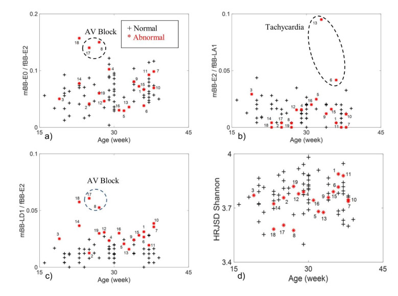
Figure 2 shows plots of some coupling patterns for the normal and the abnormal cases versus gestational age. The two single-atrium/AV block cases (ID 8, 17) revealed higher probability of occurrence for the patterns mBBI-E0/fBBI-E2 and lower probability of occurrence for the patterns mBBI-E2/fBBI-LA1 than the normal cases (Figure 2-a, b). The two tachycardia cases (ID 6, 13) showed a contrary behavior in respect to the probability of occurrence of the patterns, i.e., lower probability of occurrence of the pattern mBBI-E0/fBBI-E2 and higher probability of occurrence of the pattern mBBI-E2/fBBI-LA1.
Interestingly, the mBBI-LD1/fBBI-E2 pattern was the only HRJSD maternal-fetal coupling pattern that was significantly higher for the all abnormal cases (GAa) compared to normal cases (GA) despite the heterogeneity of abnormality ones (GAa: 0.032 ± 0.013, GA: 0.014 ± 0.007, p < 0.01 Figure 2-c). The HRJSDShannon entropy was significantly higher for the normal cases (GAa: 3.5 ± 0.09, GA: 3.6 ± 0.14, p < 0.05 Figure 2-d). The significant measures between GAa and GA groups are summarized in Table (6).
4.
Discussion
4.1. Normal pregnancies
The normal maternal-fetal cardiac coupling was mainly characterized by diminished fluctuating and alternating fetal heart rate patterns (fBBI-LD1 and fBBI-LA1) from the first to the third trimester whereas fast and strong fetal heart rate changes (fBBI-E0 and fBBI-E2) were intensified from the first to the end of the third trimester. It seems that the fetal heart rate gets more synchronized with the maternal heart rate as a stimulus from the beginning of the first trimester to the end of the third trimester. It could also be an indicator that the more matured adaptation of autonomic nervous system (ANS) casuing strong short-term maternal heart rate (mBBI-E0 and mBBI-E2) changes as external stimuli taking place much faster at the end of the third trimester than in the beginning of the first trimester. Furthermore, ANS maturation for regulating fetal heart rate changes seem to take place in the first two trimesters. Based on previous study, fetal ANS starts to develop in the 17th gestational week where the parasympathetic nerves develop rapidly in the 18th gestational week while development of the sympathetic nerves begins around the 20th gestational week, later than does that of the parasympathetic nerves, and is most rapid during the 26th to 30th gestational weeks [23].
4.2. Normal pregnancies vs. abnormal pregnancies
For the abnormal cases, some types of abnormality (particular conduction abnormalities) showed increase and some showed decrease in different maternal-fetal coupling patterns than the normal (GA) and the other types of abnormal cases. For example, the single atrium/AV-block cases showed a higher probability of occurrence of the patterns characterized by strong fetal heart rate increases and decreases (fBBI-E0 and E2) and a lower probability of occurrence of the patterns characterized by more variations (fBBI-LU1, LD1 and LA1). This might indicate the continuous elongation of the P-R interval (of the ECG) during the AV block [24].
For the tachycardia cases, a higher probability of occurrence for the patterns representing weak fetal heart rate alternation (fBBI-LA1) and a lower probability of occurrence of the patterns representing strong fetal heart rate increases (fBBI-E0) and decreases (fBBI-E2). This could have happened due to an increase in the vagal tone manifested by an increase in the beat-to-beat variability (the rmssd for the two tachycardia was 12 and 19 ms while it was 2.8±1.3 ms for the normal GA group). This could be speculated as an autonomic reflex to halt the tachycardia similar to the known vagal maneuver that is used to slow down heart rate [25].
Despite the type of abnormality, abnormal cases tended to have higher association (probability of occurrence) between maternal slow heart rate variations and fetal heart rate strong decrease (mBBI-LD1/fBBI-E2) than normal cases. This might be indicating an imbalance in ANS adaption/ modulation and could be a good marker for screening fetal cardiac wellbeing throughout the weeks of pregnancy. Measuring the degree of this coupling for developing fetuses may be useful clinical markers of healthy prenatal development and fetal cardiac anomalies. Further investigations are needed to clarify the physiological significance of the maternal–fetal heart rate coupling, and whether fetus can benefit from this specific interaction.
5.
Conclusion
HRJSD method has shown variation in coupling patterns strength that reflects the development of normal fetuses during the pregnancy period. It has also shown differences between normal and abnormal fetuses in certain coupling patterns. Further analysis with more cases of similar abnormality cases is needed to assess the accuracy of HRJSD in detecting/screening certain types of fetal abnormality by using fetal and maternal HRV.
Author contributions
AHK, SS and AV designed the study. YK collected the maternal and fetal ECG data. SS and AV applied signal processing methods and extracted coupling features. SS and HMA ran statistical analysis on results. AHK, SS, HMA and AV evaluated results of the statistical analysis. HMA wrote the main manuscript text and prepared the tables and figures and SS revised them. All authors reviewed the manuscript.
Approval, accordance and informed consent
The study protocol was approved by Tohoku University Institutional Review Board (IRB: 2015-2-80-1) and written informed consent was obtained from all subjects. All experiments were performed in accordance with relevant guidelines and regulations.
Data availability
Data used in this study will be made available upon request because we did not have any approval from ethics committee to make the data publicly available. The pregnant mothers recruited for this study did not give consent to make their data and signals available in the public domain. However, the following persons can be contacted to obtain the data under a confidentiality agreement. Dr Ahsan Khandoker (ahsan.khandoker@kustar.ac.ae); Dr Yoshitaka Kimura (ykimura@med.tohoku.ac.jp).
Conflict of interest
The authors declare no competing interests.
Funding
This study was supported by research incentive funds from Khalifa University Internal Research Fund (CIRA-2019-023).


 DownLoad: