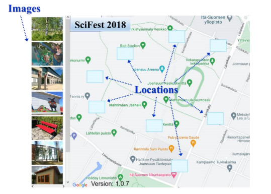
This paper presents a new class of games: location puzzle games. It combines puzzle games with the use of the geographical location. The game class is closely related to location-based games except that no physical movement in the real world is needed as in most mobile location-based games. For example, we present a game called Puzzle-Mopsi, which asks users to match a given set of images with the locations shown on the map. In addition to local knowledge, the game requires logical skills as the number of possible matches grows exponentially with the number of images. Small-scale experiments show that the players found the game interesting and that the difficulty increases with the number of targets and decreases with the player's familiarity with the area.
Citation: Pasi Fränti, Lingyi Kong. Puzzle-Mopsi: A location-puzzle game[J]. Applied Computing and Intelligence, 2023, 3(1): 1-12. doi: 10.3934/aci.2023001
This paper presents a new class of games: location puzzle games. It combines puzzle games with the use of the geographical location. The game class is closely related to location-based games except that no physical movement in the real world is needed as in most mobile location-based games. For example, we present a game called Puzzle-Mopsi, which asks users to match a given set of images with the locations shown on the map. In addition to local knowledge, the game requires logical skills as the number of possible matches grows exponentially with the number of images. Small-scale experiments show that the players found the game interesting and that the difficulty increases with the number of targets and decreases with the player's familiarity with the area.

| [1] |
P. A. Rauschnabel, A. Rossmann, M. C. tom Dieck, An adoption framework for mobile augmented reality games: The case of Pokémon Go, Comput. Human Behav., 76 (2017), 276–286. https://doi.org/10.1016/j.chb.2017.07.030 doi: 10.1016/j.chb.2017.07.030

|
| [2] |
B. E. Schlatter, A. R. Hurd, Geocaching: 21st-century Hide-and-Seek, J. Phys. Educ. Recreat. Danc., 76 (2005), 28–32. https://doi.org/10.1080/07303084.2005.10609309 doi: 10.1080/07303084.2005.10609309
|
| [3] |
M. Majorek, M. Du Vall, Ingress:An Example of a New Dimension in Entertainment, Games Cult., 11 (2016), 667–689. https://doi.org/10.1177/1555412015575833 doi: 10.1177/1555412015575833
|
| [4] |
S. Lammes, C. Wilmott, The map as playground: Location-based games as cartographical practices, Convergence, 24 (2018), 648–665. https://doi.org/10.1177/1354856516679596 doi: 10.1177/1354856516679596
|
| [5] | K. Swedlund, M. Barr, The Gilmorehill Mystery: A Location-Based Game for Campus Exploration, Int. Conf. Entertain. Comput., (2021), 236–251. Springer, Cham. https://doi.org/10.1007/978-3-030-89394-1_18 |
| [6] |
D. Spikol, M. Milrad, Combining Physical Activities and Mobile Games to Promote Novel Learning Practices, Proc. - 5th IEEE Int. Conf. Wireless, Mobile, Ubiquitous Technol. Educ. WMUTE 2008, (2008), 31–38. https://doi.org/10.1109/WMUTE.2008.37 doi: 10.1109/WMUTE.2008.37
|
| [7] |
R. Wetzel, L. Blum, L. Oppermann, Tidy City - A location-based game supported by in-situ and web-based authoring tools to enable user-created content, Found. Digit. Games 2012, FDG 2012 - Conf. Progr., (2012), 238–241. https://doi.org/10.1145/2282338.2282385 doi: 10.1145/2282338.2282385
|
| [8] |
M. Ercsey-Ravasz, Z. Toroczkai, The chaos within Sudoku, Sci. Rep., 2 (2012), 1–8. https://doi.org/10.1038/srep00725 doi: 10.1038/srep00725
|
| [9] |
A. Scott, U. Stege, I. van Rooij, Minesweeper May Not Be NP-Complete but Is Hard Nonetheless, Math. Intell., 33 (2011), 5–17. https://doi.org/10.1007/s00283-011-9256-x doi: 10.1007/s00283-011-9256-x
|
| [10] |
A. R. Strom, S. Barolo, Using the game of mastermind to teach, practice, and discuss scientific reasoning skills, PLoS Biol., 9 (2011), e1000578. https://doi.org/10.1371/journal.pbio.1000578 doi: 10.1371/journal.pbio.1000578
|
| [11] |
P. Fränti, R. Mariescu-Istodor, L. Sengupta, O-mopsi: Mobile orienteering game for sightseeing, exercising, and education, ACM T. Multim. Comput., 13 (2017), 1‒25. https://doi.org/10.1145/3115935 doi: 10.1145/3115935
|
| [12] |
C. H. Papadimitriou, The Euclidean travelling salesman problem is NP-complete, Theor. Comput. Sci., 4 (1977), 237–244. https://doi.org/10.1016/0304-3975(77)90012-3 doi: 10.1016/0304-3975(77)90012-3
|
| [13] |
M. R. Johnson, Casual Games Before Casual Games: Historicizing Paper Puzzle Games in an Era of Digital Play, Games Cult., 14 (2019), 119–138. https://doi.org/10.1177/1555412018790423 doi: 10.1177/1555412018790423
|
| [14] | V. M. Karhulahti, Puzzle is not a game! Basic structures of challenge, DiGRA 2013 - Proc. 2013 DiGRA Int. Conf. DeFragging GameStudies, 2013. |
| [15] |
M. Muller-Brockhausen, M. Preuss, A. Plaat, A New Challenge: Approaching Tetris Link with AI, IEEE Conf. Comput. Intell. Games, CIG, (2021), 1‒8. https://doi.org/10.1109/CoG52621.2021.9619044 doi: 10.1109/CoG52621.2021.9619044
|
| [16] |
K. H. Hsiao, On the structural analysis of open-keyhole puzzle locks in ancient china, Mech. Mach. Theory, 118 (2017), 168–179. https://doi.org/10.1016/j.mechmachtheory.2017.08.003 doi: 10.1016/j.mechmachtheory.2017.08.003
|
| [17] |
D. X. Zeng, M. Li, J. J. Wang, Y. L. Hou, W. J. Lu, Z. Huang, Overview of Rubik's cube and reflections on its application in mechanism, Chinese J. Mech. Eng., 31 (2018), 1‒12. https://doi.org/10.1186/s10033-018-0269-7 doi: 10.1186/s10033-018-0269-7
|
| [18] | C. T. Kong, S. M. Yiu, The Possibility of Solving a 3x3 Rubik's Cube under 3 Seconds, International Journal of Mathematical and Computational Sciences, 16 (2022), 43–51. |
| [19] |
A. Antonova, B. Bontchev, Exploring Puzzle-Based Learning for Building Effective and Motivational Maze Video Games for Education, EDULEARN19 Proc., (2019), 2425–2434. https://doi.org/10.21125/edulearn.2019.0658 doi: 10.21125/edulearn.2019.0658
|
| [20] |
O. W. S. Huang, H. N. H. Cheng, T. W. Chan, Number jigsaw puzzle: A mathematical puzzle game for facilitating players' problem-solving strategies, Proc. - Digit. 2007 First IEEE Int. Work. Digit. Game Intell. Toy Enhanc. Learn., (2007), 130–134. https://doi.org/10.1109/DIGITEL.2007.37 doi: 10.1109/DIGITEL.2007.37
|
| [21] |
D. Eppstein, Solving single-digit sudoku subproblems, Lect. Notes Comput. Sci. (including Subser. Lect. Notes Artif. Intell. Lect. Notes Bioinformatics), 7288 (2012), 142–153. https://doi.org/10.1007/978-3-642-30347-0_16 doi: 10.1007/978-3-642-30347-0_16
|
| [22] | M. Wiemker, E. Elumir, A. Clare, Escape Room Games: Can you transform an unpleasant situation into a pleasant one?, Game Based Learn., 55 (2015), 55–68. |
| [23] |
O. Ahlqvist, Location-Based Games, Int. Encycl. Geogr. People, Earth, Environ. Technol., (2016), 1–4. https://doi.org/10.1002/9781118786352.wbieg0298 doi: 10.1002/9781118786352.wbieg0298
|
| [24] |
M. Thongmak, Protecting privacy in Pokémon Go: A multigroup analysis, Technol. Soc., 70 (2022), 101999. https://doi.org/10.1016/j.techsoc.2022.101999 doi: 10.1016/j.techsoc.2022.101999
|
| [25] |
A. de Souza e Silva, R. Glover-Rijkse, A. Njathi, D. de Cunto Bueno, Playful mobilities in the Global South: A study of Pokémon Go play in Rio de Janeiro and Nairobi, New Media Soc., (2021). https://doi.org/10.1177/14614448211016400 doi: 10.1177/14614448211016400
|
| [26] |
Y. Guo, S. Agrawal, S. Peeta, I. Benedyk, Safety and health perceptions of location-based augmented reality gaming app and their implications, Accid. Anal. Prev., 161 (2021), 106354. https://doi.org/10.1016/j.aap.2021.106354 doi: 10.1016/j.aap.2021.106354
|
| [27] |
P. Alavesa, Y. Xu, Unblurring the boundary between daily life and gameplay in location-based mobile games, visual online ethnography on Pokémon GO, Behav. Inf. Technol., 41 (2022), 215–227. https://doi.org/10.1080/0144929X.2020.1825810 doi: 10.1080/0144929X.2020.1825810
|
| [28] |
H. Söbke, J. Baalsrud Hauge, I. A. Stefan, Prime Example Ingress Reframing the Pervasive Game Design Framework (PGDF), Int. J. Serious Games, 4 (2017), 39–58. https://doi.org/10.17083/ijsg.v4i2.182 doi: 10.17083/ijsg.v4i2.182
|
| [29] |
S. Laato, T. Pietarinen, S. Rauti, M. Paloheimo, N. Inaba, E. Sutinen, A review of location-based games: Do they all support exercise, social interaction and cartographical training?, CSEDU 2019 - Proc. 11th Int. Conf. Comput. Support. Educ., (2019), 616–627. https://doi.org/10.5220/0007801206160627 doi: 10.5220/0007801206160627
|
| [30] |
C. Sintoris, A. Stoica, I. Papadimitriou, N. Yiannoutsou, V. Komis, N. Avouris, MuseumScrabble: Design of a mobile game for Children's interaction with a digitally augmented cultural space, Int. J. Mob. Hum. Comput. Interact., 2 (2010), 53–71. https://doi.org/10.4018/jmhci.2010040104 doi: 10.4018/jmhci.2010040104
|
| [31] |
R. Suomela, A. Koivisto, My photos are my bullets - Using camera as the primary means of player-to-player interaction in a mobile multiplayer game, Lect. Notes Comput. Sci. (including Subser. Lect. Notes Artif. Intell. Lect. Notes Bioinformatics), 4161 (2006), 250–261. https://doi.org/10.1007/11872320_30 doi: 10.1007/11872320_30
|
| [32] |
S. Matyas, C. Matyas, C. Schlieder, P. Kiefer, H. Mitarai, M. Kamata, Designing location-based mobile games with a purpose - Collecting geospatial data with cityexplorer, Proc. 2008 Int. Conf. Adv. Comput. Entertain. Technol. ACE 2008, (2008), 244–247. https://doi.org/10.1145/1501750.1501806 doi: 10.1145/1501750.1501806
|
| [33] |
T. J. Chin, Y. You, C. Coutrix, J. H. Lim, J. P. Chevallet, L. Nigay, Mobile phone-based mixed reality: The Snap2Play game, Vis. Comput., 25 (2009), 25–37. https://doi.org/10.1007/s00371-008-0283-3 doi: 10.1007/s00371-008-0283-3
|
| [34] |
H. Tüzün, M. Yilmaz-Soylu, T. Karakuş, Y. Inal, G. Kizilkaya, The effects of computer games on primary school students' achievement and motivation in geography learning, Comput. Educ., 52 (2009), 68–77. https://doi.org/10.1016/j.compedu.2008.06.008 doi: 10.1016/j.compedu.2008.06.008
|
| [35] |
N. Nova, F. Girardin, P. Dillenbourg, Location is not enough!': An empirical study of location-awareness in mobile collaboration, Proc. - IEEE Int. Work. Wirel. Mob. Technol. Educ. WMTE 2005, 2005 (2005), 21–28. https://doi.org/10.1109/WMTE.2005.2 doi: 10.1109/WMTE.2005.2
|
| [36] | D. La Guardia, M. Arrigo, O. Di Giuseppe, A Location-Based Serious Game to Learn About the Culture, Int. Conf. Futur. Educ., (2012), 1–3. |
| [37] |
K. Vassilakis, O. Charalampakos, G. Glykokokalos, P. Kontokalou, M. Kalogiannakis, N. Vidakis, Learning by playing: An LBG for the Fortification Gates of the Venetian walls of the city of Heraklion, EAI Endorsed Trans. Creat. Technol., 5 (2018), 156773. https://doi.org/10.4108/eai.7-3-2019.156773 doi: 10.4108/eai.7-3-2019.156773
|
| [38] |
I. Jormanainen, P. Korhonen, Science festivals on Computer Science recruitment, Proc. 10th Koli Call. Int. Conf. Comput. Educ. Res. Koli Calling'10, (2010), 72–73. https://doi.org/10.1145/1930464.1930476 doi: 10.1145/1930464.1930476
|
| [39] |
A. Tabarcea, Z. Wan, K. Waga, P. Fränti, O-mopsi: Mobile orienteering game using geotagged photos, WEBIST 2013 - Proc. 9th Int. Conf. Web Inf. Syst. Technol., (2013), 300–303. https://doi.org/10.5220/0004370203000303 doi: 10.5220/0004370203000303
|
| [40] |
L. Sengupta, R. Mariescu-Istodor, P. Fränti, Planning Your Route: Where to Start?, Comput. Brain Behav., 1 (2018), 252–265. https://doi.org/10.1007/s42113-018-0018-0 doi: 10.1007/s42113-018-0018-0
|
| [41] | J. Stuckman, G.-Q. Zhang, Mastermind is NP-Complete, (2005), 1–7. |
| [42] | L. Kong, Puzzle-Mopsi: Location-based puzzle game, University of Eastern Finland, 2022. |
| [43] | N. Fazal, Radu Mariescu-Istodor, Pasi Fränti, Using Open Street Map for Content Creation in Location-Based Games, 5 (2021), 3–11. https://doi.org/10.23919/FRUCT52173.2021.9435502 |
| [44] |
L. Sengupta, P. Fränti, Comparison of eleven measures for estimating difficulty of open-loop TSP instances, Appl. Comput. Intell., 1 (2021), 1–30. https://doi.org/10.3934/aci.2021001 doi: 10.3934/aci.2021001
|


Figures(8) / Tables(1)
Pasi Fränti, Lingyi Kong. Puzzle-Mopsi: A location-puzzle game[J]. Applied Computing and Intelligence, 2023, 3(1): 1-12. doi: 10.3934/aci.2023001


 DownLoad: