Depression and Parkinson's disease: a Chicken-Egg story

Ashok Chakraborty; Anil Diwan; Ashok Chakraborty; Anil Diwan

doi:10.3934/Neuroscience.2022027

AIMS Neuroscience

2022, Volume 9, Issue 4: 479-490. doi: 10.3934/Neuroscience.2022027

Previous Article Next Article

Review

Depression and Parkinson's disease: a Chicken-Egg story

Running title:Running Title: Parkinson's disease and Depression follow each other

Ashok Chakraborty ^,,
Anil Diwan

AllExcel, Inc. Shelton, CT, USA

Received: 26 May 2022 Revised: 07 November 2022 Accepted: 11 November 2022 Published: 23 November 2022

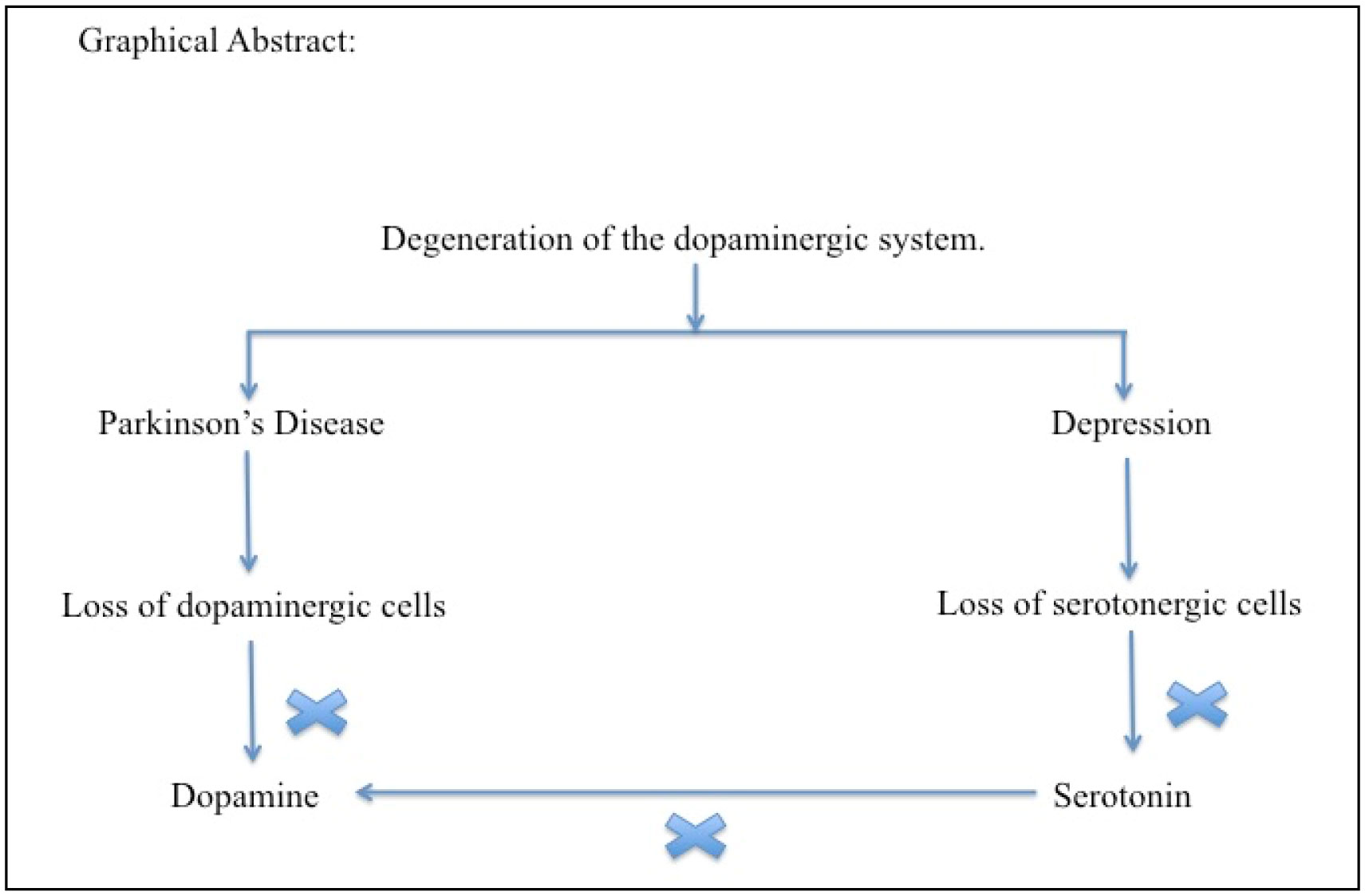
Parkinson's disease (PD) is a neurodegenerative disease, however, besides the motor symptoms, such as rest tremor, hypokinesia, postural instability and rigidity, PD patients have also non-motor symptoms, namely neuropsychiatric disorders. Apart from the required motor symptoms, psychopathological symptoms are very common and include mood disorders, anxiety disorders, hallucinations, psychosis, cognitive deterioration and dementia. The underlying pathophysiological process in PD is mainly due to the loss of dopaminergic neural cells and thereby causes the shortage of nigrostriatal dopamine content in them. In addition, it may involve other neurotransmitter systems such as the noradrenergic, serotonergic, cholinergic and noradrenergic systems as well. Depression can result from any unhealthy conditions making the diagnosis a challenging task. The manifestation of depression associated with or without PD is inadequate. The co-occurrence of depression and PD often leads to the conceptual discussion on whether depressive symptoms appear before or after PD develops. This paper will discuss the conceptual mechanism of PD and depression. Keep in mind both conditions belong to two separate entities but share some similar aspects in their pathophysiology.

Keywords:

Citation: Ashok Chakraborty, Anil Diwan. Depression and Parkinson's disease: a Chicken-Egg story[J]. AIMS Neuroscience, 2022, 9(4): 479-490. doi: 10.3934/Neuroscience.2022027

Related Papers:

[1]	Kuntha Pin, Jung Woo Han, Yunyoung Nam . Retinal diseases classification based on hybrid ensemble deep learning and optical coherence tomography images. Electronic Research Archive, 2023, 31(8): 4843-4861. doi: 10.3934/era.2023248
[2]	Peng Ren, Qunli Xia . Classification method for imbalanced LiDAR point cloud based on stack autoencoder. Electronic Research Archive, 2023, 31(6): 3453-3470. doi: 10.3934/era.2023175
[3]	Qianpeng Xiao, Changbin Shao, Sen Xu, Xibei Yang, Hualong Yu . CCkEL: Compensation-based correlated k-labelsets for classifying imbalanced multi-label data. Electronic Research Archive, 2024, 32(5): 3038-3058. doi: 10.3934/era.2024139
[4]	Tej Bahadur Shahi, Cheng-Yuan Xu, Arjun Neupane, Dayle B. Fleischfresser, Daniel J. O'Connor, Graeme C. Wright, William Guo . Peanut yield prediction with UAV multispectral imagery using a cooperative machine learning approach. Electronic Research Archive, 2023, 31(6): 3343-3361. doi: 10.3934/era.2023169
[5]	Mengke Lu, Shang Gao, Xibei Yang, Hualong Yu . Improving performance of decision threshold moving-based strategies by integrating density-based clustering technique. Electronic Research Archive, 2023, 31(5): 2501-2518. doi: 10.3934/era.2023127
[6]	Mohd. Rehan Ghazi, N. S. Raghava . Securing cloud-enabled smart cities by detecting intrusion using spark-based stacking ensemble of machine learning algorithms. Electronic Research Archive, 2024, 32(2): 1268-1307. doi: 10.3934/era.2024060
[7]	Yike Lv, Xinzhu Meng . Evolution of infectious diseases induced by epidemic prevention publicity and interaction between heterogeneous strains. Electronic Research Archive, 2024, 32(8): 4858-4886. doi: 10.3934/era.2024223
[8]	Xiaoyan Wu, Guowen Ye, Yongming Liu, Zhuanzhe Zhao, Zhibo Liu, Yu Chen . Application of Improved Jellyfish Search algorithm in Rotate Vector reducer fault diagnosis. Electronic Research Archive, 2023, 31(8): 4882-4906. doi: 10.3934/era.2023250
[9]	Boshuo Geng, Jianxiao Ma, Shaohu Zhang . Ensemble deep learning-based lane-changing behavior prediction of manually driven vehicles in mixed traffic environments. Electronic Research Archive, 2023, 31(10): 6216-6235. doi: 10.3934/era.2023315
[10]	Chetan Swarup, Kamred Udham Singh, Ankit Kumar, Saroj Kumar Pandey, Neeraj varshney, Teekam Singh . Brain tumor detection using CNN, AlexNet & GoogLeNet ensembling learning approaches. Electronic Research Archive, 2023, 31(5): 2900-2924. doi: 10.3934/era.2023146

Abstract

1. Introduction

Learning from class imbalanced data is a hotspot and challenging issue in the field of machine learning ^[1,2]. Also, we note that the class imbalance problem exists widely in real-world applications, including biology data processing ^[3], business data analysis ^[4], industry fault detection ^[5], face recognition ^[6] and crime linkage discovery ^[7]. In these applications, the users generally focus on the minority class that has less training instances than the other classes. However, the conventional supervised learning algorithms always expect to minimize the overall training errors, and hence it is inevitable to favor the majority class but sacrifice the performance of the minority class.

Over the past two decades, many learning algorithms for addressing the imbalanced classification problem have been proposed. The methods mainly include sampling ^{[8,9,10,11,12,13,14,15,16]}, cost-sensitive learning ^[17,18,19], threshold-moving ^[20,21,22], one-class learning ^[23] and ensemble learning ^{[24,25,26,27,28,29,30,31]} or multiple classifiers system ^{[32,33,34,35,36,37,38,39]}. Sampling is a data preprocessing strategy that is used to add the minority instances (oversampling) or remove the majority examples (undersampling) to balance the training set, further satisfying the learning rule of the conventional supervised learning algorithms. Cost-sensitive learning assigns higher penalty weights for minority instances to force the learning algorithms to pay more attention to the minority class. Threshold-moving is a post-processing solution which empirically or adaptively tunes the decision threshold to push the classification hyperplane towards the majority class. One-class learning, which describes the boundary of one class by merely training on the instances belonging to that class, is generally used to address a highly imbalanced problem. Ensemble learning aims to utilize the other class imbalance learning methods, e.g., sampling, cost-sensitive-cost learning or threshold-moving, to combine with the emerging ensemble learning paradigms, e.g., bagging or boosting, for classifying imbalanced data. In comparison to those single models, ensemble learning is expected to greatly improve the classification performance, especially the generalization ability, on class imbalanced data. In view of the merits of ensemble learning, it has been widely studied and adopted in the context of imbalanced data classification.

As we know, to make an ensemble classifier be effective, we should consider two key factors. The first one is that the performance of each base classifier should be not very poor, and the other one is that all base classifiers contained in an ensemble should be diverse as far as possible ^[40]. For the first factor, most class imbalance ensemble learning algorithms can guarantee it well by assigning excellently distributed training subsets and designating a robust supervised learning algorithm to train each base classifier. Meanwhile, for the second factor, i.e., diversity, many ensemble learning algorithms cannot satisfy it well, as most of them acquire diversity only by perturbing distributions of instances or costs in each training subset. Actually, only when there is a balance between the single performance and the group diversity, the corresponding ensemble model could present the strongest performance ^[38].

In this study, we focus on how to further improve the diversity of ensemble classifiers and how to find the best tradeoff between single performance and group diversity. For the first problem, we profit from the idea of ^[39] to combine multiple different sampling algorithms and multiple different types of classifiers to construct a heterogeneous ensemble learning algorithm. As indicated in ^[39], perturbing instances and classifiers simultaneously can help provide more diversity for an ensemble and meanwhile can improve the quality of the ensemble. As for the second problem, considering that one cannot simply estimate the potential and effect of each base classifier in ensemble by its single performance, an evolutionary genetic algorithm is adopted to adaptively select a high-quality combination of base classifiers for making the decision. According to the many could be better than all theory ^[41], the selective ensemble strategy must be helpful for searching a better tradeoff between single performance and group diversity. We call the proposed ensemble learning algorithm Selective Evolutionary Heterogeneous Ensemble, which can be called SEHE in brief. To verify the effectiveness and feasibility of the proposed SEHE algorithm, we compare it with lots of state-of-the-art class imbalance ensemble learning algorithms on 42 imbalanced data sets acquired in the Keel data repository ^[42] and UCI machine learning repository ^[43], and the results show the superiority of SEHE.

The main contribution in this study is combining the ideas of the heterogeneous ensemble and the selective ensemble to improve the performance of class imbalanced learning. To our best knowledge, it is the first time integrating these two ideas for addressing the class imbalanced learning problem. It not only increases diversity production but also helps to find the best tradeoff between single performance and group diversity

The remainder of this paper is organized as follows. Section 2 reviews the related work about class imbalance ensemble learning. Section 3 describes the proposed SEHE algorithm and its framework in detail. In Section 4, the experimental results and analysis are presented. Finally, Section 5 concludes this study and indicates the future research directions.

2. Related work

As mentioned above, lots of different techniques and solutions have been proposed to solve the class imbalance problem during the past two decades, in which the ensemble learning is most successful and popular to address such problem ^[1,2]. The general idea of class imbalance ensemble learning is to combine a single class imbalanced learning technique, e.g., sampling, cost-sensitive learning or threshold-moving, with one of the Bagging or Boosting ensemble learning paradigms for achieving the aim of improving the generalization capability of the classification model. Here, the adoption of a single technique aims to acquire an approximately unbiased base classifier, while the adoption of an ensemble aims to promote the robustness of the decision model.

Some primitive class imbalance ensemble learning algorithms, including UnderBagging ^[24], OverBagging ^[37], SMOTEBagging ^[37], RUSBoost ^[33], SMOTEBoost ^[25], EUSBoost ^[28], Asymmetric Bagging ^[36], etc., directly combine a simple undersampling or oversampling algorithm with a Bagging or Boosting ensemble framework. The merit of these algorithms lies in that they are simple and easily implemented. However, they produce diversity only by sampling different data subsets. It is clear that when adopting an undersampling strategy to generate training subsets, the diversity of training subsets could be highlighted, but the performance of each single base learning model could not be safely guaranteed. Meanwhile, oversampling safeguards the performance of a single model but always hurts the group diversity. Yu et al. ^[38] indicated that when and only when there exists an approximate tradeoff between single performance and group diversity, the quality of the ensemble could be maximized. They integrated several techniques, including feature selection, feature subspace, asymmetric bagging, into an ensemble algorithm called asBagging-FSS for classifying high-dimensional imbalanced biomedicine data. In contrast to Asymmetric Bagging ^[36], the asBagging-FSS simultaneously enhances the group diversity by inserting disturbances in feature space and the single performance by adding a feature selection procedure. However, the solution might be ineffective on low-dimensional class imbalanced data.

Another group of class imbalance ensemble learning algorithms consider coupling instance costs together with ensemble learning. In fact, the cost of an instance can be naturally combined with the Boosting ensemble learning paradigm. Some well-known algorithms integrating both cost-sensitive learning and Boosting include AdaCost ^[27], AdaC1 ^[34], AdaC2 ^[34] and AdaC3 ^[34]. These ensemble solutions gradually focus on classifying those difficult instances by the way of iterative feedback. In such fashion, the diversity between two continuous base classifiers can be seen as the variance of cost distributions.

Several algorithms also combine the threshold-moving technique with the Bagging ensemble learning paradigm, such as PT-Bagging ^[26] and EnSVM-OTHR ^[20]. Specifically, the PT-Bagging produces diversity only relying on bootstrap strategy which is a natural step in Bagging, while the EnSVM-OTHR adopts both bootstrap and a small random disturbance happening on the adjusted threshold to acquire diverse base classifiers.

To enhance the performance of a single model in an ensemble, some previous studies utilize the ensemble learning model to represent the single model, i.e., the algorithm can be seen as an ensemble of an ensemble. Such cases include EasyEnsemble ^[30], BalanceCascade ^[30] and GIR series algorithms ^[35]. Specifically, in GIR series algorithms, two sampling approaches convert the class imbalance problem into several balanced sub-problems for training the classifiers, and in each sub-problem, several weak classifiers are respectively trained by using Boosting method and finally combined by Bagging. These two-level ensemble algorithms ignore the effect of diversity, and hence the performance improvement is generally restricted.

In recent several years, more and more researchers began to focus on studying how to promote diversity in an ensemble. The strategies of enhancing ensemble diversity include evolutionary strategy ^[29,31] and heterogeneous ensemble ^[39]. Roshan and Asadi ^[31] adopted a popular evolutionary multi-objective optimization algorithm called NSGA-II to synchronously optimize the three following goals: class imbalance ratio IR in each bag, group diversity in ensemble and AUC performance metric. Lim et al. ^[29] presented a novel cluster-based synthetic oversampling (CSO) algorithm and integrated its five hyper-parameters in each bag together to implement chromosome encoding, finally taking advantage of a genetic algorithm (GA) to determine and produce training subsets. Due to the number of data to generate, the clustering method, the number of clusters, the number of nearest neighbors within each cluster for oversampling and the oversampling method are different in different bags, so there exists a significant diversity among those generated training subsets. Zefrehi and Altincay ^[39] investigated the possibility of integrating both heterogeneous sampling strategies and classification models to enhance diversity in an ensemble. A significant performance improvement has been observed by adopting heterogeneous classifiers in contrast to using homogeneous classifiers. Meanwhile, when the number of heterogeneous classifiers increases from 1 to 5, the performance of the ensemble model can continuously increase.

According to the reviews above, it is not difficult to observe that there are two major challenges for the class imbalance ensemble learning technique. The first one is how to further improve the group diversity, and the second one is how to achieve an approximately excellent tradeoff between single performance and group diversity. In this study, we wish to simultaneously focus on these two problems.

3. Methods

In this section, we first introduce the heterogeneous class imbalance ensemble learning method, and then on this basis, a selective evolutionary heterogeneous class imbalanced ensemble learning algorithm is described in detail.

3.1. Heterogeneous class imbalance ensemble learning framework

As we know, developing a successful ensemble learning method should simultaneously focus on the two following conditions: the quality of single base learning model and the group diversity among different base learning models ^[40]. It is not difficult to generate high-quality single classifiers; however, it is a difficult task guaranteeing the generated base classifiers to be diverse enough. The reason lies in that diversity, as an abstract notion, is difficult to accurately measure. In addition, the methods of producing and/or enhancing diversity are generally naïve. In Bagging, it always adopts a bootstrap technique to produce diverse training subsets for acquiring diversity, and hence it guarantees to produce 36.8% diverse training instances between two different subsets in theory ^[44]. In contrast, the Boosting acquires diverse training subsets by disturbing the distribution of training instances or the weights of training instances ^[45], which is totally uncontrolled in practical applications. Random forest ^[46] and random subspace ^[47] enhance the diversity of training subsets by disturbing both instance space and feature space, but the diversity promotion would be limited by the dimension of the feature space. That is to say, if the training data is low-dimension, we could not significantly improve the diversity of training subsets by these two methods.

All methods mentioned above utilize data-level disturbance to produce diversity. However, it is noteworthy that the classifier level can produce diversity for an ensemble, too. That means the diversity source can be associated with adopting multiple types of classifiers. In general, we call this strategy heterogeneous ensemble. Several previous works have indicated that the diversity among heterogeneous members is significantly higher than that of homogeneous ones ^[48,49], and the heterogeneous ensemble always performs better than any one single member ^[50,51]. As for class imbalance learning, an ensemble algorithm combining heterogeneous sampling and heterogeneous classifiers had also been proposed by Zefrehi and Altincay ^[39] and had acquired improving classification results in comparison to some popular class imbalance ensemble learning algorithms. Profiting from the idea of the HeteroEn algorithm proposed in ^[39], we propose a heterogeneous ensemble (HE) algorithm for addressing the class imbalance learning problem.

Let Φ denote the class imbalanced training data set, and S = {s₁, s₂, …, s_L} and K = {k₁, k₂, …, k_N} respectively denote the set including L different sampling algorithms and the set containing N diverse types of classifiers. Then, we can produce L*N diverse combinations of training subsets and classification approaches, where each combination has one of two differences at the data level and classifier level from any other combination at least. In HE, the most popular and simplest decision rule, i.e., majority voting, is adopted to combine decisions of all base classifiers. The flow path of the HE algorithm is described below.

Algorithm 1: HE algorithm
Input: A class imbalanced training set Φ, a sampling approaches set S = {s₁, s₂, …, s_L}, a classification methods set K = {k₁, k₂, …, k_N}
Output: An ensemble classifier set E = {C₁₁, C₁₂, …, C_1N, C₂₁, C₂₂, …, C_2N, ……, C_L1, C_L2…C_LN}
Procedure:
1. Initialize E = ϕ;
2. for i = 1: L
3. for j = 1:N
4. generate a training subset Φ_ij by adopting the sampling algorithm s_i acting on the training set Φ;
5. train a base classifier C_ij on the training subset Φ_ij by adopting the classification method k_j;
6. put C_ij into E;
7. end
8. end

A more intuitive description about the flow path of the HE algorithm can be observed in Figure 1.

Figure 1. Description for the flow path of the HE algorithm.

DownLoad: Full-Size Img PowerPoint

It is worthy to note that although both the HeteroEn algorithm proposed in ^[39] and our HE algorithm adopt the same construction, that is, the combination of diverse sampling approaches and heterogeneous classifiers to construct an ensemble, there is a significant difference between them. The difference lies in that the HeteroEn algorithm integrates the heterogeneous combination into Bagging and Boosting ensemble learning frameworks, while our proposed HE algorithm only produces L*N base classifiers, equal to the number of combinations constructed on the data level and classifier level. The merits of such way are two-fold: 1) It would not generate excessively redundant base classifiers which lack enough diversity with each other in the ensemble; 2) the size of the ensemble could be restricted in a small scale to help reduce time and storage consumption.

To make HE be effective, we also need to consider which sampling approaches and classification algorithms should be put into S and K, respectively. Obviously, to guarantee the quality of a single base classifier, each sampling and each classification algorithm in HE should be robust. Furthermore, to enhance the diversity, both sampling algorithms and classification models should be based on different theoretical rules and inherent assumptions. According to these two criterions, we select seven sampling approaches (including three undersampling algorithms: RUS ^[9], UFFDFR ^[12] and MPBU ^[13]; and four oversampling algorithms: ROS ^[9], SMOTE ^[11], MWMOTE ^[8] and GA-SMOTE ^[16]) and six classification models to constitute S and K in HE, respectively. These heterogeneous methods are shown in Table 1. In practical applications, the combination of these methods is not constant, and thus the users are encouraged to add and remove any sampling approach or classification model in this list.

Table 1. Sampling approaches and classification methods used in HE.

sampling approach		classification method
s₁	RUS ^[9]	k₁	decision tree (CART)
s₂	UFFDFR ^[12]	k₂	K-nearest neighbors (KNN)
s₃	MPBU ^[13]	k₃	support vector machine (SVM) with Gaussian kernel
s₄	ROS ^[9]	k₄	extreme learning machine (ELM) with sigmoid activation function
s₅	SMOTE ^[11]	k₅	logistic regression (LR)
s₆	MWMOTE ^[8]	k₆	naïve Bayes classifier (NB)
s₇	GA-SMOTE ^[16]

| Show Table

DownLoad: CSV

3.2. Selective evolutionary heterogeneous class imbalance ensemble learning algorithm

In HE, although we have safeguarded the performance of the ensemble by adopting robust and diverse sampling approaches and classification methods, there is still a huge potential to further improve the quality of the ensemble. This is because each classification method has its specific inherent assumption, which causes it to perform well on some data but perform poorly on some other data. This phenomenon has been observed by many previous works ^[8,14,16]. Therefore, it is necessary to remove some low-quality single base classifiers for further enhancing the quality of the ensemble. However, considering that diversity is an abstract notion, it is difficult to directly estimate the effect and potential of any one base classifier in HE, and thus it can be regarded as a sophisticated optimization problem. This is consistent with the idea of selective ensemble ^[41], i.e., many could be better than all.

To solve the optimization problem above, we refer the idea in ^[41] to conduct a procedure of selective ensemble on HE by using an evolutionary genetic algorithm. The proposed algorithm is called selective evolutionary heterogeneous ensemble, which can be also called SEHE in brief. It is clear that the SEHE is an adaptive algorithm to avoid estimating the quality of each base classifier and the diversity among them.

The reason for selecting the genetic algorithm is that the optimization problem in SEHE is discrete, which is specifically appropriate for use with this optimization technique. There are several key conditions and parameters, which are chromosome encoding strategy, fitness function, population size, crossover factor, mutation factor and the termination condition, that should be seriously considered in a genetic algorithm ^[52]. In our proposed SEHE algorithm, the chromosome encoding is organized as a vector of length L*N to represent all base classifiers. In each position of the chromosome, it adopts a binary coding, where 1 indicates the corresponding base classifier joining into the final ensemble, while 0 expresses that the corresponding one should be excluded from the final ensemble. Each chromosome denotes an alternative of selective ensemble. As for the fitness function that is used to evaluate the quality of each selective ensemble solution, we consider that it should be directly associated with a performance evaluation metric. Here, we adopt a combination of two popular class imbalance learning performance evaluation metrics, i.e., F1-measure and G-mean, as the fitness function f. In particular, the F1-measure originating from F-measure can be calculated as below:

F - measure = \frac{(1 + β^{2}) \times recall \times precision}{β^{2} \times recall + precision}

${\text{F - measure = }}\frac{{(1 + {\beta ^2}) \times {\text{recall}} \times {\text{precision}}}}{{{\beta ^2} \times {\text{recall + precision}}}}$

(1)

where β is a parameter denoting the relative importance between precision and recall. In general, β is set to be 1, and then the metric is transformed to be the widely used F1-measure, i.e.,

F1 - measure = \frac{2 \times recall \times precision}{recall + precision}

${\text{F1 - measure = }}\frac{{2 \times {\text{recall}} \times {\text{precision}}}}{{{\text{recall + precision}}}}$

(2)

G-mean can be calculated as below:

G - mean = \sqrt{TPR \times TNR}

${\text{G - mean = }}\sqrt {{\text{TPR}} \times {\text{TNR}}}$

(3)

where TPR and TNR denote the true positive rate and true negative rate, respectively. Thus, the G-mean metric can be regarded as a tradeoff between TPR and TNR. Based on the F1-measure and G-mean, the fitness function f can be calculated as follows.

f = \frac{1}{2} \times F1 - measure + \frac{1}{2} \times G - mean

$f{\text{ = }}\frac{1}{2} \times {\text{F1 - measure}} + \frac{1}{2} \times {\text{G - mean}}$

(4)

It is obvious that the fitness function f represents an impartial tradeoff between F1-measure and G-mean.

In addition, to keep the tradeoff between the quality of solution and running time consumption, the population size and terminal iterative times are empirically suggested to be designated as 50 and 30, respectively. Furthermore, to accelerate the exploration process, the crossover factor and mutation factor are respectively set to be 1.0 and 0.1 in SEHE. That means all parents conduct crossover operation to generate their offspring, and random 10% of positions of all chromosomes transform their coding values.

The flow path of the proposed evolutionary algorithm is presented as below.

Algorithm 2: Evolutionary algorithm
Input: An ensemble classifier set E which includes L*N base classifiers, the population size parameter N_pop, a crossover factor N_c, a mutation factor N_m, the terminal iterative times N_s
Output: A selective ensemble set SE
Procedure:
1. Initialize a binary vector V_best with length L*N randomly;
2. Initialize a variance f_best, which is used to reserve the current best fitness value, as 0;
3. Initialize N_pop chromosomes with the length L*N using binary coding randomly;
4. for i = 1: N_s
5. transform each chromosome to an ensemble according to its coder mapping on E, and estimate its quality by the fitness function, then compare it with f_best, if there exists a better fitness value, it would be used to replace f_best, and meanwhile the corresponding chromosome would be used to update V_best;
6. end
7. decode V_best on E to acquire SE.
8. end

In addition, we note that the fitness function of evolutionary algorithm associates with both F1-measure and G-mean metrics, and then if both the training procedure of HE and the calculation of fitness of evolutionary algorithm are conducted directly on the original training set Φ, the selected combination of base classifiers might be overfit. To solve the problem, we adopt an internal five-fold cross validation strategy in our SEHE algorithm, in which the original training set E is averagely divided into five non-overlapping subsets Φ₁, Φ₂, Φ₃, Φ₄ and Φ₅. First, we conduct a five-round iterative operation in which at each round, four subsets are integrated as the internal training set, and the remaining one is used as the internal verifying set. Then, on each internal training set, we conduct the HE algorithm to produce L*N classifiers. That means 5*L*N classifiers are generated in total. Next, for each chromosome in SEHE, its fitness is estimated five times, in which for the ith time, the corresponding classifiers trained on the ith internal training set are used to evaluate the chromosome's fitness on the ith internal verifying set. Furthermore, we adopt the average of the five results as the fitness of the chromosome. Finally, to avoid wasting the training instances, it is required to retrain the best combination of classifiers on the original training set Φ after finishing the evolutionary procedure. Based on this rule, the flow path of the SEHE algorithm can be described as follows.

From the flow path of the SEHE algorithm, it is not difficult to observe that it is implemented by a two-level training procedure, where the first level runs in a five-fold cross validation environment to search for the best combination of sampling approaches and classification methods, while the second level takes charge of retraining this combination on the original training set to produce the selective ensemble result. Due to the adoption of a two-level training mode and evolutionary algorithm, it is inevitable that SEHE is a time-consuming algorithm.

Algorithm 3: SEHE algorithm
Input: A class imbalance training set Φ, a sampling approaches set S = {s₁, s₂, …, s_L}, a classification methods set K = {k₁, k₂, …, k_N}, the population size parameter N_pop, a crossover factor N_c, a mutation factor N_m, the terminal iterative times N_s
Output: A selective ensemble set SE
Procedure:
1. divide randomly Φ into five average subsets Φ₁, Φ₂, Φ₃, Φ₄ and Φ₅;
2. for i = 1:5
3. integrate all training subsets except Φ_i as training set Ψ_i;
4. call HE algorithms to produce an ensemble classifiers set E_i on Ψ_i;
5. produce the output of each base classifier in E_i on each instance in the verifying set Φ_i, and record them;
6. end
7. call evolutionary algorithm to get a binary vector indicating which combinations of sampling approaches and classification methods should be reserved;
8. adopt the reserved combinations to retrain a selective ensemble set SE on Φ.

4. Experiments and analysis

4.1. Experimental data description

We collected 42 imbalanced data sets, including 30 ones from Keel data repository ^[42] and 12 ones from UCI machine learning repository ^[43], to verify the effectiveness and superiority of the proposed SEHE algorithm. Specifically, these datasets have different numbers of instances, numbers of features and class imbalance ratios. The information about these data sets is described in Table 2 in detail.

Table 2. Description about the used class imbalanced data sets in this study, where #Instances and #Features denote respectively the number of instances and features contained in the corresponding dataset, and IR denotes the class imbalance ratio, which is calculated by the number of majority instances / the number of minority instances.

Dataset	#Instances	#Features	IR	Dataset	#Instances	#Features	IR
glass1	214	9	1.82	ecoli-0-6-7_vs_5	220	6	10.00
wisconsin	683	9	1.86	led7digit-0-2-4-5-6-7-8-9_vs_1	443	7	10.97
pima	768	8	1.87	ecoli-0-1_vs_5	240	6	11.00
haberman	306	3	2.78	shuttle-6_vs_2-3	230	9	22.00
vehicle1	846	18	2.90	flare-F	1066	11	23.79
new-thyroid1	215	5	5.14	winequality-red-4	1599	11	29.17
yeast3	1484	8	8.10	shuttle-2_vs_5	3316	9	66.67
ecoli3	336	7	8.60	poker-8-9_vs_5	2075	10	82.00
vowel0	988	13	9.98	poker-8_vs_6	1477	10	85.88
yeast-1_vs_7	459	7	14.30	banknote	1372	4	1.25
ecoli4	336	7	15.80	ctgC5	2126	21	28.50
abalone9-18	731	8	16.40	ctgN1vsN3	2126	21	3.50
shuttle-c2-vs-c4	129	9	20.90	ctgN2	2126	21	6.20
yeast4	1484	8	28.10	ctgN3	2126	21	11.10
yeast5	1484	8	32.73	wilt	4839	5	17.50
abalone19	4174	8	129.44	mfeatmor01	2000	6	4.00
ecoli-0-3-4_vs_5	200	7	9.00	mfeatmor012	2000	6	2.30
ecoli-0-6-7_vs_3-5	222	7	9.09	seeds2v13	210	7	2.00
yeast-0-3-5-9_vs_7-8	506	8	9.12	segment1	2310	19	6.00
yeast-0-3-5-9_vs_7-8	1004	8	9.14	segment12	2310	19	2.50
ecoli-0-1_vs_2-3-5	244	7	9.17	segment123	2310	19	1.30

| Show Table

DownLoad: CSV

4.2. Experimental settings

To estimate whether the proposed SEHE algorithm is effective and feasible, it is widely compared with some popular and state-of-the-art class imbalance ensemble learning algorithms, including UnderBagging ^[24], OverBagging ^[37], SMOTEBagging ^[37], RUSBoost ^[33], SMOTEBoost ^[25], EUSBoost ^[28], EnSVM-OTHR ^[20], EasyEnsemble ^[30], BalanceCascade ^[30], GIREnUS ^[35], 2Obj* ^[31], ECO-Ensemble ^[29], HeteroEn ^[39] and our proposed HE algorithm. Considering that the parameter settings in any algorithm could affect its performance and further influence the impartiality of experiment comparisons, we adopted the recommended parameter settings referred to in each study as default ones. For examples, in ^[35], we selected GIREnUS, which had been indicated to perform better than its partner, i.e., GIREnOS, while in ^[31], we adopted the 2Obj* version that outperforms two other algorithm versions. As for the number of base classifiers, all Bagging- and Boosting- based algorithms are uniformly designated as 100 and 20, respectively. In addition, the base classifier types in each ensemble algorithm adopted the default ones used in the corresponding study. For our proposed HE and SEHE algorithm, all sampling algorithms contained in them used the default parameters recommended in the corresponding references, and the classification algorithms used the following parameter settings: The KNN adopted a default parameter k = 5, the SVM used a RBF kernel function with σ = 0.01 and the penalty factor C = 1, the ELM adopted the sigmoid activation function with L = 50 hidden nodes, and the LR used L2 regularization with a default penalty factor C = 1. To guarantee the impartiality of experiments, if some other ensemble learning algorithms have adopted one or several sampling or classification algorithms that are the same as the ones used in our proposed algorithm, they have been designated the same parameter settings.

Both F1-measure and G-mean metrics which have been used to evaluate the fitness in our proposed SEHE algorithm are also selected as the performance evaluation metric for comparing various ensemble algorithms. In particular, both F1-metric and G-mean have been shown as the most popular metrics to evaluate the quality of a class imbalance learning algorithm.

Finally, to impartially compare the quality of all comparative algorithms, 10 random runs' external five-fold cross validation is conducted for each algorithm, and the average performance of the corresponding 50 validated results is used to represent its final result.

4.3. Results and discussion

Tables 3 and 4 present the comparative results of 15 ensemble learning algorithms in terms of F1-measure and G-mean metrics, respectively. Specifically, on each data set, the best result has been highlighted in boldface.

Table 3. F1-measure results of 15 comparative algorithms, where on each data set, the best result has been highlighted in bold.

Dataset	Under Bagging	Over Bagging	SMOTE Bagging	RUSBoost	SMOTE Boost	EUSBoost	EnSVM -OTHR	Easy Ensemble	Balance Cascade	GIREnUS	2Obj*	ECO -Ensemble	HeteroEn	HE	SEHE
glass1	0.6179	0.6418	0.6566	0.6531	0.6479	0.6710	0.7022	0.6937	0.6819	0.7074	0.7196	0.7338	0.7292	0.7231	0.7479
wisconsin	0.9496	0.9501	0.9532	0.9458	0.9526	0.9531	0.9368	0.9444	0.9496	0.9537	0.9486	0.9529	0.9501	0.9529	0.9685
pima	0.6074	0.6291	0.6399	0.6518	0.6436	0.6457	0.6706	0.6619	0.6538	0.6560	0.6489	0.6917	0.6742	0.6721	0.6898
haberman	0.4310	0.4036	0.4117	0.4425	0.4328	0.4679	0.4658	0.4631	0.4254	0.4738	0.4699	0.4852	0.4798	0.4881	0.5122
vehicle1	0.6829	0.6473	0.6428	0.6716	0.6632	0.6811	0.6793	0.6627	0.6519	0.6521	0.7044	0.6759	0.6792	0.6721	0.7022
new-thyroid1	0.9275	0.9310	0.9288	0.9219	0.9468	0.9390	0.9426	0.9410	0.9272	0.9587	0.9446	0.9510	0.9451	0.9439	0.9517
yeast3	0.6866	0.6922	0.7014	0.7250	0.7033	0.7315	0.7446	0.7361	0.7410	0.7398	0.7316	0.7425	0.7355	0.7398	0.7461
ecoli3	0.5632	0.5791	0.6318	0.6007	0.6101	0.6049	0.6251	0.5735	0.5816	0.5835	0.5961	0.6032	0.6397	0.6381	0.6441
vowel0	0.9489	0.9876	0.9941	0.9774	0.9986	0.9826	0.9978	0.9598	0.9689	0.9936	0.9972	1.0000	0.9983	0.9973	1.0000
yeast-1_vs_7	0.2816	0.2459	0.4109	0.3828	0.4350	0.3744	0.3610	0.2969	0.2871	0.3980	0.3792	0.4160	0.3967	0.4159	0.4287
ecoli4	0.6491	0.7387	0.7519	0.6393	0.7275	0.7080	0.7441	0.6146	0.7269	0.7484	0.7175	0.7290	0.7448	0.7641	0.7548
abalone9-18	0.3353	0.3798	0.4314	0.3722	0.3918	0.3816	0.4277	0.2934	0.2987	0.3970	0.4052	0.4329	0.4320	0.4388	0.4530
shuttle-c2-vs-c4	0.9964	0.9981	1.0000	0.9981	1.0000	0.9993	0.9976	0.9952	0.9971	0.9994	1.0000	0.9972	0.9991	1.0000	1.0000
yeast4	0.2798	0.3362	0.3517	0.3394	0.3707	0.3239	0.3949	0.2875	0.2987	0.3708	0.3646	0.3802	0.3569	0.3694	0.3743
yeast5	0.5967	0.6652	0.6743	0.5969	0.6837	0.6345	0.6874	0.5350	0.5989	0.6947	0.6528	0.6777	0.6931	0.6895	0.6933
abalone19	0.0372	0.0991	0.0869	0.0417	0.1132	0.0507	0.0962	0.0487	0.0396	0.1133	0.1521	0.1312	0.1479	0.1455	0.1752
ecoli-0-3-4_vs_5	0.7109	0.7983	0.8109	0.7329	0.8086	0.7751	0.8108	0.6954	0.7374	0.7930	0.8028	0.8039	0.8184	0.7999	0.8481
ecoli-0-6-7_vs_3-5	0.5819	0.6343	0.6420	0.5927	0.6588	0.6447	0.6736	0.5210	0.6001	0.6542	0.6571	0.6848	0.6352	0.6572	0.6791
yeast-0-3-5-9_vs_7-8	0.2933	0.3231	0.3490	0.2815	0.3140	0.3392	0.3431	0.3089	0.3076	0.3418	0.3396	0.3210	0.3317	0.3396	0.3991
yeast-0-3-5-9_vs_7-8	0.6956	0.7722	0.7630	0.6717	0.7448	0.7134	0.7520	0.6837	0.7474	0.7541	0.7498	0.7526	0.7279	0.7579	0.7890
ecoli-0-1_vs_2-3-5	0.5549	0.6627	0.6788	0.5610	0.6472	0.6081	0.6654	0.6344	0.6290	0.6708	0.6587	0.6842	0.6738	0.6688	0.7223
ecoli-0-6-7_vs_5	0.5345	0.6860	0.7438	0.6633	0.7297	0.7515	0.7337	0.6125	0.7120	0.6995	0.7498	0.7355	0.7378	0.7394	0.7511
led7digit-0-2-4-5-6-7-8-9_vs_1	0.6627	0.7413	0.7427	0.6580	0.7336	0.7189	0.7355	0.6528	0.7066	0.7209	0.7515	0.7320	0.7458	0.7468	0.7515
ecoli-0-1_vs_5	0.7440	0.7752	0.7836	0.7506	0.7878	0.7441	0.7642	0.6784	0.7043	0.7531	0.7752	0.7807	0.7735	0.7742	0.7835
shuttle-6_vs_2-3	0.8929	0.7304	0.7543	0.8891	0.7984	0.8894	0.8906	0.8814	0.8839	0.8539	0.8901	0.8872	0.8756	0.8795	0.9194
flare-F	0.1909	0.2542	0.2798	0.2590	0.2711	0.2433	0.2677	0.2516	0.2702	0.2710	0.2688	0.2854	0.2860	0.2991	0.3796
winequality-red-4	0.1277	0.1792	0.2098	0.1744	0.1811	0.1795	0.1811	0.1342	0.0970	0.1979	0.1594	0.1945	0.1986	0.2333	0.2691
shuttle-2_vs_5	1.0000	0.9951	1.0000	0.9729	0.9982	1.0000	1.0000	0.9684	0.9797	0.9968	0.9981	1.0000	0.9952	0.9954	1.0000
poker-8-9_vs_5	0.0372	0.0661	0.0971	0.0422	0.1157	0.0679	0.1011	0.0385	0.0406	0.0920	0.1008	0.1106	0.1033	0.1176	0.1795
poker-8_vs_6	0.2906	0.6790	0.6929	0.2409	0.6508	0.4411	0.4076	0.1919	0.2143	0.5080	0.6945	0.6991	0.6876	0.6734	0.7394
banknote	0.9828	0.9816	0.9830	0.9901	0.9749	0.9826	0.9724	0.9849	0.9751	0.9810	0.9886	0.9815	0.9843	0.9799	0.9896
ctgC5	0.2820	0.3144	0.3462	0.2517	0.3727	0.2342	0.3109	0.3519	0.3442	0.3031	0.3572	0.3648	0.3528	0.3591	0.4327
ctgN1vsN3	0.6542	0.7310	0.7479	0.6968	0.7444	0.7991	0.7580	0.7374	0.7511	0.7332	0.7546	0.7590	0.7376	0.7521	0.7986
ctgN2	0.6378	0.7436	0.7387	0.7115	0.7220	0.7159	0.7034	0.7519	0.7226	0.7258	0.7196	0.7364	0.7419	0.7644	0.7428
ctgN3	0.7476	0.8095	0.7964	0.7555	0.7858	0.7336	0.7686	0.7587	0.7462	0.7680	0.7904	0.7725	0.7531	0.7549	0.8073
wilt	0.5625	0.6991	0.7415	0.6423	0.7404	0.6985	0.7840	0.7379	0.6581	0.8132	0.7310	0.7796	0.7529	0.7522	0.8461
mfeatmor01	0.9089	0.9735	0.9818	0.9527	0.9886	0.9532	0.9897	0.9436	0.9528	0.9789	0.9901	0.9592	0.9301	0.9459	0.9711
mfeatmor012	0.8546	0.8369	0.8226	0.8990	0.8467	0.8971	0.8858	0.8442	0.8325	0.8790	0.8687	0.8884	0.8628	0.8844	0.9122
seeds2v13	0.9776	0.9664	0.9685	0.9702	0.9573	0.9696	0.9668	0.9794	0.9801	0.9642	0.9715	0.9733	0.9598	0.9696	0.9798
segment1	0.8806	0.9428	0.9335	0.9010	0.9552	0.9336	0.9344	0.9522	0.9121	0.9258	0.9306	0.9357	0.9281	0.9194	0.9479
segment12	0.9562	0.9314	0.9210	0.9668	0.9506	0.9632	0.9545	0.9619	0.9454	0.9508	0.9612	0.9675	0.9449	0.9491	0.9677
segment123	0.9986	0.9847	0.9859	0.9987	0.9856	0.9981	1.0000	0.9992	0.9992	0.9983	0.9869	1.0000	0.9906	0.9984	1.0000

| Show Table

DownLoad: CSV

Table 4. G-mean results of 15 comparative algorithms, where on each data set, the best result has been highlighted in bold.

Dataset	Under Bagging	Over Bagging	SMOTE Bagging	RUSBoost	SMOTE Boost	EUSBoost	EnSVM -OTHR	Easy Ensemble	Balance Cascade	GIREnUS	2Obj*	ECO -Ensemble	HeteroEn	HE	SEHE
glass1	0.7211	0.7202	0.7198	0.7454	0.7219	0.7418	0.7529	0.7622	0.7619	0.7588	0.7641	0.7832	0.7699	0.7701	0.8109
wisconsin	0.9796	0.9701	0.9732	0.9769	0.9680	0.9745	0.9761	0.9687	0.9594	0.9732	0.9858	0.9761	0.9752	0.9747	0.9830
pima	0.6733	0.6566	0.6721	0.6831	0.6702	0.6801	0.7673	0.7328	0.7285	0.7271	0.7166	0.7330	0.7575	0.7520	0.7793
haberman	0.6010	0.5994	0.6004	0.6002	0.6118	0.6233	0.6219	0.6258	0.6146	0.6375	0.5998	0.6425	0.6333	0.6379	0.6412
vehicle1	0.7858	0.7741	0.7759	0.7901	0.7722	0.7910	0.7853	0.7766	0.7692	0.7581	0.7834	0.8022	0.7931	0.8018	0.8356
new-thyroid1	0.9792	0.9801	0.9847	0.9818	0.9836	0.9790	0.9829	0.9715	0.9718	0.9844	0.9901	0.9774	0.9855	0.9882	0.9899
yeast3	0.8993	0.8899	0.8706	0.8944	0.9052	0.8911	0.9237	0.8901	0.8877	0.9018	0.9134	0.9075	0.8969	0.8993	0.9105
ecoli3	0.8580	0.8681	0.8706	0.8478	0.8644	0.8590	0.8647	0.8760	0.8791	0.8632	0.8661	0.8744	0.8709	0.8776	0.8924
vowel0	0.9978	0.9963	0.9981	0.9972	0.9950	0.9981	1.0000	0.9935	0.9962	1.0000	0.9971	1.0000	0.9994	0.9991	1.0000
yeast-1_vs_7	0.5678	0.6882	0.7109	0.5945	0.7208	0.7044	0.6786	0.7430	0.7238	0.7196	0.7200	0.6959	0.7006	0.7159	0.7455
ecoli4	0.9196	0.8998	0.9106	0.9042	0.9119	0.9208	0.9198	0.9304	0.9196	0.9211	0.9307	0.9256	0.9388	0.9306	0.9329
abalone9-18	0.6495	0.6784	0.6513	0.6690	0.6755	0.6821	0.7492	0.7326	0.7419	0.7430	0.7374	0.7513	0.7333	0.7420	0.7764
shuttle-c2-vs-c4	0.9971	0.9984	1.0000	0.9975	1.0000	0.9995	0.9977	0.9941	0.9986	0.9997	1.0000	0.9982	0.9995	1.0000	1.0000
yeast4	0.8139	0.8057	0.8236	0.8294	0.8175	0.8277	0.8310	0.8194	0.8196	0.8079	0.8221	0.8174	0.8395	0.8358	0.8379
yeast5	0.9535	0.9457	0.9674	0.9521	0.9443	0.9576	0.9495	0.9478	0.9406	0.9528	0.9663	0.9712	0.9591	0.9544	0.9642
abalone19	0.3447	0.7240	0.7461	0.3290	0.6973	0.7276	0.5969	0.7085	0.4919	0.6738	0.7092	0.7329	0.7170	0.7181	0.7702
ecoli-0-3-4_vs_5	0.8781	0.8857	0.8796	0.8981	0.8848	0.8932	0.8921	0.8830	0.8829	0.8990	0.8998	0.8776	0.8939	0.8901	0.8957
ecoli-0-6-7_vs_3-5	0.8306	0.7998	0.8081	0.8272	0.8198	0.8255	0.8551	0.8030	0.8212	0.8187	0.8190	0.8464	0.8211	0.8186	0.8539
yeast-0-3-5-9_vs_7-8	0.6997	0.5687	0.5868	0.6739	0.5710	0.6845	0.6861	0.6932	0.6911	0.6954	0.6878	0.6759	0.6922	0.6878	0.7154
yeast-0-3-5-9_vs_7-8	0.8874	0.9028	0.9012	0.8966	0.8998	0.8775	0.8964	0.8981	0.8942	0.8911	0.8886	0.8932	0.8897	0.8933	0.8959
ecoli-0-1_vs_2-3-5	0.8377	0.8119	0.8088	0.8394	0.8299	0.8301	0.8442	0.8527	0.8504	0.8425	0.8501	0.8499	0.8455	0.8479	0.8697
ecoli-0-6-7_vs_5	0.8000	0.8642	0.8591	0.8320	0.8529	0.8617	0.8832	0.8653	0.8724	0.8695	0.8610	0.8736	0.8575	0.8531	0.8792
led7digit-0-2-4-5-6-7-8-9_vs_1	0.8534	0.8631	0.8670	0.8498	0.8692	0.8506	0.8772	0.8650	0.8762	0.8696	0.8779	0.8699	0.8858	0.8744	0.8821
ecoli-0-1_vs_5	0.8850	0.8952	0.8926	0.8901	0.8974	0.8833	0.8906	0.8864	0.8732	0.8830	0.8868	0.8953	0.8862	0.8934	0.9195
shuttle-6_vs_2-3	0.8586	0.7760	0.7793	0.8228	0.7896	0.8499	0.8934	0.8820	0.8959	0.8876	0.9030	0.9123	0.8896	0.8867	0.9095
flare-F	0.8218	0.7477	0.7652	0.8333	0.7501	0.8198	0.6744	0.8219	0.7946	0.8079	0.8139	0.8448	0.7989	0.8016	0.8337
winequality-red-4	0.5919	0.6732	0.6673	0.5792	0.6545	0.5808	0.6273	0.5898	0.5170	0.6914	0.6632	0.6500	0.6705	0.6829	0.7173
shuttle-2_vs_5	1.0000	0.9982	1.0000	0.9711	0.9976	1.0000	1.0000	0.9774	0.9823	0.9954	0.9987	1.0000	0.9965	0.9988	1.0000
poker-8-9_vs_5	0.3317	0.6053	0.6149	0.3140	0.5782	0.3438	0.5562	0.3710	0.3929	0.4618	0.4491	0.5312	0.4700	0.4854	0.6157
poker-8_vs_6	0.5252	0.7410	0.7299	0.5740	0.7318	0.5237	0.7098	0.6536	0.6790	0.7492	0.7008	0.7129	0.7190	0.7152	0.7733
banknote	0.9876	0.9810	0.9809	0.9913	0.9804	0.9821	0.9856	0.9830	0.9777	0.9822	0.9896	0.9811	0.9834	0.9791	0.9850
ctgC5	0.5134	0.6658	0.6233	0.5730	0.6419	0.5099	0.5858	0.5736	0.6297	0.6419	0.6322	0.6785	0.6412	0.6430	0.6859
ctgN1vsN3	0.8297	0.8170	0.8254	0.8137	0.8350	0.8445	0.8454	0.8361	0.8299	0.8317	0.8471	0.8360	0.8338	0.8415	0.8447
ctgN2	0.8052	0.7969	0.8011	0.7994	0.8138	0.7876	0.8452	0.8092	0.7956	0.8004	0.8123	0.8223	0.7964	0.8558	0.8770
ctgN3	0.8211	0.8732	0.8536	0.8341	0.8840	0.8109	0.8444	0.8277	0.8309	0.8650	0.8233	0.8766	0.8427	0.8501	0.8766
wilt	0.7691	0.7038	0.6852	0.7222	0.7001	0.7559	0.7981	0.7226	0.7028	0.8006	0.7304	0.7578	0.7449	0.7611	0.7999
mfeatmor01	0.9521	0.9815	0.9874	0.9662	0.9901	0.9633	0.9884	0.9601	0.9732	0.9807	0.9874	0.9663	0.9406	0.9535	0.9715
mfeatmor012	0.8998	0.8227	0.8376	0.9015	0.8778	0.9192	0.9135	0.9004	0.8858	0.9030	0.8564	0.9002	0.8568	0.8774	0.9323
seeds2v13	0.9855	0.9724	0.9789	0.9802	0.9693	0.9891	0.9868	0.9780	0.9876	0.9905	0.9872	0.9901	0.9701	0.9743	0.9856
segment1	0.9423	0.9637	0.9716	0.9332	0.9630	0.9236	0.9579	0.9411	0.9619	0.9690	0.9848	0.9597	0.9481	0.9577	0.9700
segment12	0.9701	0.9539	0.9611	0.9678	0.9555	0.9690	0.9772	0.9571	0.9580	0.9747	0.9689	0.9677	0.9704	0.9708	0.9882
segment123	0.9991	0.9897	0.9879	0.9994	0.9834	0.9990	1.0000	0.9995	0.9994	0.9989	0.9881	1.0000	0.9935	0.9991	1.0000

| Show Table

DownLoad: CSV

From the results in Tables 3 and 4, it is not difficult to observe that our proposed SEHE algorithm outperforms all other competitors, as it produces best F1-measure result on 24 data sets and best G-mean result on 22 data sets, which are much more than the number of the best results acquired by adopting other class imbalance ensemble learning algorithms. We note that no matter if it is on those data sets with low class imbalance ratio or on highly imbalanced data sets, our proposed SEHE algorithm can produce good classification results. We believe that it associates with the two following reasons: 1) The combination of heterogeneous sampling methods and heterogeneous classification models provides enough diversity for constructing ensemble learning model, and 2) the evolutionary selection procedure in SEHE algorithm adaptively meets the demands of data distribution well. Therefore, we can say that the proposed SEHE algorithm is a robust, flexible and self-adaptive class imbalance learning algorithm.

Another interesting conclusion that can be observed from the results in Tables 3 and 4 is that several state-of-the-art algorithms proposed in recent several years, including EnSVM-OTHR, GIREnUS, 2Obj*, ECO-Ensemble and HeteroEn, generally perform better than those previously popular algorithms. Of course, in contrast to those simple ensembles, these state-of-the-art algorithms often have more sophisticated constructions, and hence their training procedures are more complex, too.

We also observe that the proposed SEHE algorithm performs obviously better than the HE algorithm on almost all data sets, showing the correctness of adopting selective ensemble strategy, again. We believe that in comparison to aggregating all base classifiers, adaptively selecting some of them would be helpful for searching for a better tradeoff between single performance and group diversity.

Furthermore, we are curious which combinations between sampling approaches and classification methods perform better in HE. On each data set, we scanned the average performance of F1-measure and G-mean throughout all combinations, and the best combination was recorded based on the feedback of 10 random runs' external five-fold cross validation. Further, the top 10 combinations are presented in Table 5. One could make the following conclusion from the results in Table 5: Combining one of those sophisticated sampling approaches, e.g., MWMOTE, MPBU, UFFDFR or GA-SMOTE, and one of those robust classification methods, e.g., Support Vector Machine or Extreme Learning Machine, it is easier to produce excellent classification performance.

Table 5. Top 10 combinations between single sampling approach and classification method in HE.

Rank		Combination	# data sets performing best
1	MPBU + Support Vector Machine		7
2	UFFDFR + Logistic Regression		5
3	MWMOTE + Extreme Learning Machine		4
4	MWMOTE + Support Vector Machine		3
5	UFFDER + CART		3
6	GA-SMOTE + Support Vector Machine		2
7	MPBU + KNN		2
8	MWMOTE + Support Vector Machine		2
9	GA-SMOTE + Extreme Learning Machine		2
10	MPBU + Extreme Learning Machine		2

| Show Table

DownLoad: CSV

Furthermore, we investigated an important issue, that is, how many base classifiers have been selected to organize the ensemble in our proposed SEHE algorithm? Figure 2 shows the average number of selected base classifiers in SEHE based on 50 independent runs on each data set. In Figure 2, we observed that on most data sets, SEHE integrates no more than 20 base classifiers to make final decision but produces robust results, which verifies the assumption that SEHE could adaptively find the trade-off between single quality and group diversity, again.

Figure 2. Average number of selected base classifiers in SEHE on each data set, where the number on the horizontal axis corresponds to the order of the data set in Table 2.

DownLoad: Full-Size Img PowerPoint

4.4. Significance analysis

Next, the Nemenyi test ^[53,54] is used to observe whether there exist some actual differences between the proposed SEHE algorithm and the other comparative algorithms in statistics. Specifically, the critical difference (CD) metric is used to show the differences among various algorithms. Figure 3 shows the CD diagram at a standard level of significance, α = 0.05, where the average ranking of each algorithm is marked along the axis (higher rankings to the left). In a CD diagram, if a group of algorithms are not significantly different, then these algorithms will be connected by a thick line.

In Figure 3, we observed that our proposed SEHE algorithm has acquired the lowest average rankings 1.7976 on F1-measure and 2.3571 on G-mean, which show that it is the best one among all comparative algorithms on both metrics. At a standard level of significance, α = 0.05, SEHE significantly outperforms its competitors except ECO-Ensemble on F1-measure metric. Therefore, we have to say that on the F1-metric at least, in contrast to the ECO-Ensemble algorithm, our proposed SEHE algorithm has not presented a significant superiority. In addition, another conclusion can be drawn from the results in Figure 3, i.e., several state-of-the-art algorithms proposed in several recent years generally perform better than those previously popular algorithms.

Figure 3. CD diagrams of various comparative algorithms at a standard level of significance, α = 0.05.

DownLoad: Full-Size Img PowerPoint

4.5. Performance improvement with two baselines

To make clear how much improvement the proposed SEHE algorithm has acquired, we also compared it with the two following baselines: One is the performance yielded by the best base classifier in HE, and the other one is the performance produced by HE. The percentages of performance improvement compared with the two baselines in terms of F1-measure and G-mean metrics are respectively presented in Figure 4.

Figure 4. Percentage of performance improvement of SEHE in comparison with two baselines: HE and the best base classifier in HE, on each data set.

DownLoad: Full-Size Img PowerPoint

Figure 4 shows that on most data sets, the proposed SEHE algorithms can improve classification performance in comparison with two baselines to some extent, which indicates the necessity of adopting a selective ensemble, again. Meanwhile, we observed an interesting phenomenon, that is, on most data sets, the HE algorithm performs poorer than its best member (base classifier). This is acceptable, because in a practical application, it cannot foresee the best combination of sampling method and classification model. In contrast to directly integrating heterogeneous methods, the model selection is obviously a more complex task.

4.6. Ablation study

Finally, we designed two groups of ablation experiments to make clear the effect of adopting diverse sampling approaches and heterogeneous classifiers in SEHE, respectively. We tuned the ablation at the data level and classifier level, respectively. That is to say, for each test, we only reserve either one data-level or one classifier-level method in SEHE, whereas the other level remains stable. For example, if the ablation associates with SMOTE, then all other sampling algorithms would be removed, but the classifier level still maintains six heterogeneous classifiers. Considering that the ablation reduces the ensemble size and further causes an impartial comparison, we utilized the bootstrap technique before sampling to guarantee that a total number of 42 diverse base classifiers can be generated. A pairwise t-test at 5% significance level was adopted to compare SEHE with its ablation algorithm, and further the numbers of wins/ties/losses throughout all 42 data sets were recorded, respectively.

Table 6. Statistical comparison between SEHE and its data-level ablation algorithm based on a pairwise t-test at 5% significance level.

Ablation comparison	F1-measure			G-mean
Ablation comparison	Win	Tie	Loss	Win	Tie	Loss
SEHE vs. SEHE_RUS	15	26	1	14	25	3
SEHE vs. SEHE_UFFDFR	13	28	1	14	28	0
SEHE vs. SEHE_MPBU	11	29	2	15	26	1
SEHE vs. SEHE_ROS	10	31	1	12	28	2
SEHE vs. SEHE_SMOTE	7	33	2	9	29	4
SEHE vs. SEHE_MWMOTE	6	34	2	10	29	3
SEHE vs. SEHE_GA-SMOTE	6	32	4	8	33	1

| Show Table

DownLoad: CSV

Table 7. Statistical comparison between SEHE and its classifier-level ablation algorithm based on a pairwise t-test at 5% significance level.

Ablation comparison	F1-measure			G-mean
Ablation comparison	Win	Tie	Loss	Win	Tie	Loss
SEHE vs. SEHE_CART	17	25	0	19	22	1
SEHE vs. SEHE_KNN	20	21	1	23	19	0
SEHE vs. SEHE_SVM	15	22	5	17	22	3
SEHE vs. SEHE_ELM	13	26	3	15	24	3
SEHE vs. SEHE_LR	18	24	0	21	20	1
SEHE vs. SEHE_NB	25	17	0	23	18	1

| Show Table

DownLoad: CSV

Tables 6 and 7 provide the results of ablation experiments at data level and classifier level, respectively. Specifically, each ablation algorithm was still conducted by 10 random runs' external five-fold cross validation. The results show that reducing diversity at data level influences less the classification performance than tuning the classifier level. In other words, the adoption of heterogeneous classifiers contributes significantly more for the success of our SEHE algorithm, which illustrates that the ensemble of heterogeneous classifiers is helpful for reducing the bias of a single classifier and enhancing group diversity of ensemble, again.

5. Conclusions

In this study, a selective evolutionary heterogeneous ensemble algorithm has been proposed to address the class imbalance learning problem. First, a group of different sampling approaches run on the original training data to acquire multiple diverse balanced training subsets. Then, each subset is trained on multiple different types of classifiers, further generating some diverse base classifiers. Next, a selective ensemble procedure relying on the evolutionary algorithm is conducted to search for the best combination of base classifiers. By lots of comparative experiments, the proposed SEHE algorithm shows a superior performance in comparison to some state-of-the-art class imbalance ensemble learning algorithms.

From the experimental results, several major conclusions could be safely drawn as follows:

1) Disturbing the data level and the classifier level both help to enhance ensemble diversity, but the disturbance at the classifier level contributes significantly more.

2) Many are really better than all: Adaptively selecting a few base classifiers always performs better than aggregating all.

3) The best base classifier often outperforms the HE, but in most cases, it performs poorer than the SEHE.

4) SEHE is a flexible, robust and competitive algorithm to solve the class imbalance learning problem in real-world applications.

In future work, the issue of how to decrease the time-complexity of the SEHE algorithm will be investigated. The performance variation of SEHE by extending the library of sampling and classification methods will be observed in future study, too. Additionally, we state that although in this study, the SEHE has not been verified on a multi-class imbalanced learning problem, it is indeed compatible for both binary and multi-class classification problems when and only when all embedded sampling algorithms are simultaneously appropriate for these two problems. Therefore, extending the current SEHE version to the multi-class classification problem for estimating its effectiveness and superiority will also be studied in future work.

Acknowledgments

This work was supported in part by the National Natural Science Foundation of China under Grant No. 62076215.

Conflict of interest

The authors declare there is no conflict of interest.

Acknowledgments

We acknowledge all our colleagues and secretaries for their help during the preparation of the manuscript and providing all the relevant information. Thanks are due to Ms. Bethany Pond, a Chemist at AllExcel, Inc. for the English corrections.

Author contributions

Both of the authors contributed equally to preparing this article, reading and approving the final manuscript.

Conflict of interest

Both of the authors declare that the research was conducted in the absence of any commercial or financial relationships that could be construed as a potential conflict of interest.

References

[1]	Ray Chaudhuri K, Healy DG, Schapira AHV (2006) Non-motor symptoms of Parkinson's disease: diagnosis and management. Lancet Neurol 5: 235-245. https://doi.org/10.1016/S1474-4422(06)70373-8
[2]	Klein C, Westenberger A (2012) Genetics of Parkinson's disease. Cold Spring Harb Perspect Med 2: a008888. https://doi.org/10.1101/cshperspect.a008888
[3]	Parkinson's Disease: Causes, Symptoms, and Treatments. Available from: https://www.nia.nih.gov/health/parkinsons-disease.
[4]	World Health OrganizationDepression: Fact Sheet (2017). Available from: http://www.who.int/mediacentre/factsheets/fs369/en.
[5]	(2000) American Psychiatric AssociationDiagnostic and statistical manual of mental disorders (DSM-IV-TR). Washington, DC: American Psychiatric Association. https://doi.org/10.1002/9780470479216.corpsy0271
[6]	Hornykiewicz O (1975) Brain monoamines and parkinsonism. Natl Inst Drug Abuse Res 11: 13-21. https://doi.org/10.1037/e472122004-001
[7]	Jellinger K (1986) An overview of morphological changes in Parkinson's disease. Adv Neurol 45: 1-18.
[8]	Hantz P, Cardoc-Davies G, Cardoc-Davies T, et al. (1994) Depression in Parkinson's disease. Am J Psychiatry 151: 1010-1014. https://doi.org/10.1176/ajp.151.7.1010
[9]	Tandberg E, Larsen JP, Aarsland D, et al. (1996) The occurrence of depression in Parkinson's disease; a community based study. Arch Neurol 53: 175-179. https://doi.org/10.1001/archneur.1996.00550020087019
[10]	Beekman ATF, Copeland JRM, Prince MJ (1999) Review of community prevalence of depression in later life. Br J Psychiatry 174: 307-311. https://doi.org/10.1192/bjp.174.4.307
[11]	Reijnders JSAM, Ehrt U, Weber WEJ, et al. (2008) A systematic review of prevalence studies of depression in Parkinson's disease. Movement Disord 23: 183-189. https://doi.org/10.1002/mds.21803
[12]	Mayeux R (1990) The serotonergic hypothesis for depression in Parkinson's disease. Adv Neurol 53: 163-166.
[13]	Van Praag HM, De Haen S (1979) Central serotonergic metabolism and frequency of depression. Psychiatr Res 1: 219-224. https://doi.org/10.1016/0165-1781(79)90002-7
[14]	Baquero M, Martin N (2015) Depressive symptoms in neurodegenerative diseases. World J Clin Cases 3: 682-693. https://doi.org/10.12998/wjcc.v3.i8.682
[15]	Hemmerle AM, Herman JP, Seroogy KB (2012) Stress, depression and Parkinson's disease. Exp Neurol 233: 79-86. https://doi.org/10.1016/j.expneurol.2011.09.035
[16]	Van Praag HM, Asnis GM, Kahn RS (1990) Monoamines and abnormal behaviour: a multi-aminergic perspective. Br J Psychiatry 157: 723-734. https://doi.org/10.1192/bjp.157.5.723
[17]	Hobson P, Holden A, Meara J (1990) Measuring the impact of Parkinson's disease with the Parkinson's Disease Quality of Life questionnaire. Age Ageing 28: 341-346. https://doi.org/10.1093/ageing/28.4.341
[18]	Liu CY, Wang SJ, Fuh JL, et al. (1997) The correlation of depression with functional ability in Parkinson's disease. J Neurol 244: 493-498. https://doi.org/10.1007/s004150050131
[19]	(2000) American Psychiatric AssociationPractice guideline for major depressive disorder in adults. American Psychiatric Association practice guidelines for the treatment of psychiatric disorder. Washington, DC: American Psychiatric Association 413-495.
[20]	Fibiger HC (1984) The neurobiological substrates of depression in Parkinson's disease: a hypothesis. Can J Neurol Sci 11: 105-107. https://doi.org/10.1017/S0317167100046230
[21]	Gonul AS, Aksu M (1999) SSRI-induced parkinsonism may be an early sign of future Parkinson's disease. J Clin Psychiatry 60: 410. https://doi.org/10.4088/JCP.v60n0611d
[22]	Mayeux R, Stern Y, Cote L, et al. (1984) Altered serotonin metabolism in depressed patients with Parkinson's disease. Neurology 34: 642-646. https://doi.org/10.1212/WNL.34.5.642
[23]	Schuurman AG, Van den Akker M, Ensinck KTJL, et al. (2002) Increased risk of Parkinson's disease after depression: a retrospective cohort study. Neurology 58: 1501-1504. https://doi.org/10.1212/WNL.58.10.1501
[24]	Nilsson FM, Kessing LV, Bolwig TG (2001) Increased risk of developing Parkinson's disease for patients with major affective disorder: a register study. Acta Psychiatr Scand 104: 380-386. https://doi.org/10.1034/j.1600-0447.2001.00372.x
[25]	McEwen BS (2003) Mood disorders and allostatic load. Biol Psychiatry 54: 200-207. https://doi.org/10.1016/S0006-3223(03)00177-X
[26]	Cole SA, Woodard JL, Juncos JL, et al. (1996) Depression and disability in Parkinson's disease. J Neuropsychiatry Clin Neurosci 8: 20-25. https://doi.org/10.1176/jnp.8.1.20
[27]	Santamaria J, Tolosa ES, Valles A, et al. (1986) Mental depression in untreated Parkinson's disease of recent onset. Adv Neurol 45: 443-446.
[28]	Schrag A, Jahanshahi M, Quinn NP (2001) What contributes to depression in Parkinson's disease?. Psychol Med 31: 65-73. https://doi.org/10.1017/S0033291799003141
[29]	Starkstein S, Preziosi TJ, Bolduc PL, et al. (1990) Depression in Parkinson's disease. J Nerv Ment Dis 178: 27-31. https://doi.org/10.1097/00005053-199001000-00005
[30]	Tandberg E, Larsen JP, Aarsland D, et al. (1997) Risk factors for depression in Parkinson's disease. Arch Neurol 54: 625-630. https://doi.org/10.1001/archneur.1997.00550170097020
[31]	Rektorova I, Rektor I, Bares M, et al. (2003) Pramipexole and per-golide in the treatment of depression in Parkinson's disease: a national multicentre prospective randomized study. Eur J Neurol 10: 399-406. https://doi.org/10.1046/j.1468-1331.2003.00612.x
[32]	Corrigan MH, Denehan AQ, Wright CE, et al. (2000) Comparison of pramipexole, fluoxetine, and placebo in patients with major depression. Depress Anxiety 11: 58-65. https://doi.org/10.1002/(SICI)1520-6394(2000)11:2<58::AID-DA2>3.0.CO;2-H
[33]	De Battista C, Solvason HB, Heilig Breen JA, et al. (2000) Pramipexole augmentation of a selective serotonin reuptake inhibitor in the treatment of depression. J Clin Psychopharmacol 20: 274-275. https://doi.org/10.1097/00004714-200004000-00029
[34]	Mayeux R, Stern Y, Cote L, et al. (1984) Altered serotonin metabolism in depressed patients with Parkinson's disease. Neurology 34: 642-646. https://doi.org/10.1212/WNL.34.5.642
[35]	Kitada T, Asakawa S, Hattori N, et al. (1998) Mutations in the parkin gene cause autosomal recessive juvenile parkinsonism. Nature 392: 605-8. https://doi.org/10.1038/33416
[36]	D'Souza T, Rajkumar A (2020) Systematic review of genetic variants associated with cognitive impairment and depressive symptoms in Parkinson's disease. Acta Neuropsychiatrica 32: 10-22. https://doi.org/10.1017/neu.2019.28
[37]	Jo S, Kim SO, Park KW, et al. (2021) The role of APOE in cognitive trajectories and motor decline in Parkinson's disease. Sci Rep 11: 7819. https://doi.org/10.1038/s41598-021-86483-w
[38]	Herbert J, Ban M, Brown GW, et al. (2012) Interaction between the BDNF gene Val/66/Met polymorphism and morning cortisol levels as a predictor of depression in adult women. Br J Psychiatry 201: 313-9. https://doi.org/10.1192/bjp.bp.111.107037
[39]	Chakraborty A, Diwan A (2022) A genetic abnormalities behind the PD, and its therapeutic intervention. Neurol Curr Res 2: 1012.
[40]	Levinson DF (2006) The Genetics of Depression: A Review. Biol Psychiat 60: 84-92. https://doi.org/10.1016/j.biopsych.2005.08.024
[41]	Sia M-W, Foo J-N, Saffari S-E, et al. (2021) Polygenic Risk Scores in a Prospective Parkinson's Disease Cohort. Movement Disord 36: 2936-2940. https://doi.org/10.1002/mds.28761
[42]	Maria S, Bondarenko EA, Slominsky PA (2018) Genetics factors in major depression disease. Front Psychiatry 9: 334. https://doi.org/10.3389/fpsyt.2018.00334
[43]	Pezzoli G, Cereda E (2013) Exposure to pesticides or solvents and risk of Parkinson disease. Neurology 80: 2035. https://doi.org/10.1212/WNL.0b013e318294b3c8
[44]	Gamache P-L, Roux-Dubois N, Provencher P, et al. (2017) Professional exposure to pesticides and heavy metals hastens Parkinson Disease onset (P6.008). Neurology 88: P6.008.
[45]	Elbaz A, Clavel J, Rathouz PJ, et al. (2009) Professional exposure to pesticides and Parkinson disease. Ann Neurol 66: 494-504. https://doi.org/10.1002/ana.21717
[46]	Pouchieu C, Piel C, Carles C, et al. (2018) Pesticide use in agriculture and Parkinson's disease in the AGRICAN cohort study. Int J Epidemiol 47: 299-310. https://doi.org/10.1093/ije/dyx225
[47]	Castillo S, Muñoz P, Behrens MI, et al. (2017) On the role of mining exposure in epigenetic effects in Parkinson's disease. Neurotox Res 32: 172-4. https://doi.org/10.1007/s12640-017-9736-7
[48]	Willis AW, Evanoff BA, Lian M, et al. (2010) Metal emissions and urban incident Parkinson disease: a community health study of medicare beneficiaries by using geographic information systems. Am J Epidemiol 172: 1357-63. https://doi.org/10.1093/aje/kwq303
[49]	Palacios N (2017) Air pollution and Parkinson's disease – evidence and future directions. Rev Environ Health 32: 303-13. https://doi.org/10.1515/reveh-2017-0009
[50]	Ritz B, Lee P-C, Hansen J, et al. (2016) Traffic-related air pollution and Parkinson's disease in Denmark: a case–control study. Environ Health Perspect 124: 351-6. https://doi.org/10.1289/ehp.1409313
[51]	Finkelstein MM, Jerrett M (2007) A study of the relationships between Parkinson's disease and markers of traffic-derived and environmental manganese air pollution in two Canadian cities. Environ Res 104: 420-32. https://doi.org/10.1016/j.envres.2007.03.002
[52]	Todd G, Pearson-Dennett V, Wilcox RA, et al. (2016) Adults with a history of illicit amphetamine use exhibit abnormal substantia nigra morphology and parkinsonism. Parkinsonism Relat Disord 25: 27-32. https://doi.org/10.1016/j.parkreldis.2016.02.019
[53]	Todd G, Noyes C, Flavel SC, et al. (2013) Illicit stimulant use is associated with abnormal substantia nigra morphology in humans. PLoS ONE 8: e56438. https://doi.org/10.1371/journal.pone.0056438
[54]	Mursaleen LR, Stamford JA (2016) Drugs of abuse and Parkinson's disease. Prog Neuropsychopharmacol Biol Psychiatry 64: 209-17. https://doi.org/10.1016/j.pnpbp.2015.03.013
[55]	Remes O, Mendes JF, Templeton P (2021) Biological, Psychological, and Social Determinants of Depression: A Review of Recent Literature. Brain Sci 11: 1633. https://doi.org/10.3390/brainsci11121633
[56]	Schrempft S, Jackowska M, Hamer M, et al. (2019) Associations between social isolation, loneliness, and objective physical activity in older men and women. BMC Public Health 19: 74. https://doi.org/10.1186/s12889-019-6424-y
[57]	Depression. Parkinson's Foundation. Available from: https://www.parkinson.org›non-movement-symptoms
[58]	Ishihara L, Brayne C (2006) A systematic review of depression and mental illness preceding Parkinson's disease. Acta Neurol Scand 113: 211-20. https://doi.org/10.1111/j.1600-0404.2006.00579.x
[59]	NIH: National Institute of Mental HealthDepression. Available from: https://www.nimh.nih.gov/health/publications/depression
[60]	Parkinson's FoundationDepression. https://www.parkinson.org/understanding-parkinsons/symptoms/non-movement-symptoms/depression
[61]	Leentjens AF, Van den Akker M, Metsemakers JF, et al. (2003) Higher incidence of depression preceding the onset of Parkinson's disease: a register study. Mov Disord 18: 414-8. https://doi.org/10.1002/mds.10387
[62]	Looi JC, Matis M, Ruzich MJ (2005) Conceptualization of depression in Parkinson's disease. Neuropsychiatr Dis Treat 1: 135-43. https://doi.org/10.2147/nedt.1.2.135.61051
[63]	Anand A, Charney DS (2000) Norepinephrine dysfunction in depression. J Clin Psychiatry 61: 16-24.
[64]	American Parkinson Disease AssociationDepression in Parkinson's. Available from: https://www.apdaparkinson.org/what-is parkinsons/symptoms/depression/
[65]	American Parkinson Disease AssociationDepression and Parkinson's disease. Available from: https://d2icp22po6iej.cloudfront.net/wp-content/uploads/2017/02/APDA1709-Supplement-Depression-D4V1.pdf
[66]	Marsh L (2013) Depression and Parkinson's disease: current knowledge. Curr Neurol Neurosci Rep 13: 409. https://doi.org/10.1007/s11910-013-0409-5
[67]	Michael J Fox Foundation for Parkinson's Research. Depression and Anxiety. Available from: https://www.michaeljfox.org/news/depression-anxiety
[68]	Parkinson's FoundationDepression. Available from: https://www.parkinson.org/Understanding-Parkinsons/Symptoms/Non-Movement-Symptoms/Depression
[69]	Mayeux R, Stern Y, Williams JBW, et al. (1986) Clinical and biochemical features of depression in Parkinson's disease. Am J Psychiatry 43: 756-9. https://doi.org/10.1176/ajp.143.6.756
[70]	Kostic VS, Djuricic BM, Covickovic-Sternic N, et al. (1987) Depression and Parkinson's disease: possible role of serotonergic mechanisms. J Neurol 234: 94-96. https://doi.org/10.1007/BF00314109
[71]	Placebo study.Imipramine in Treatment of Parkinsonism: a Double-blind Placebo Study. Br BMJ (1965) 2: 33-34. https://doi.org/10.1136/bmj.2.5452.33
[72]	Laitinen L (1969) Desipramine in treatment of Parkinson's disease. Acta Neurol Scand 45: 109-113. https://doi.org/10.1111/j.1600-0404.1969.tb01224.x
[73]	Anderson J, Aabro E, Gulmann N, et al. (1980) Anti-depressive treatment in Parkinson's disease: a controlled trial of the effect of nortriptyline in patients with Parkinson's disease treated with L-dopa. Acta Neurol Scand 62: 210-19. https://doi.org/10.1111/j.1600-0404.1980.tb03028.x
[74]	Goetz CG, Tanner CM, Klawans HL (1984) Bupropion in Parkinson's disease. Neurology 34: 1092-1094. https://doi.org/10.1212/WNL.34.8.1092
[75]	Klaassen T, Verhey FRJ, Sneijders GHJ, et al. (1995) Treatment of depression in Parkinson's disease: a meta-analysis. J Neuropsychiatry Clin Neurosci 7: 281-286. https://doi.org/10.1176/jnp.7.3.281

This article has been cited by:

1.	Qi Dai, Long-hui Wang, Kai-long Xu, Tony Du, Li-fang Chen, Class-overlap detection based on heterogeneous clustering ensemble for multi-class imbalance problem, 2024, 255, 09574174, 124558, 10.1016/j.eswa.2024.124558
2.	Qianpeng Xiao, Changbin Shao, Sen Xu, Xibei Yang, Hualong Yu, CCkEL: Compensation-based correlated k-labelsets for classifying imbalanced multi-label data, 2024, 32, 2688-1594, 3038, 10.3934/era.2024139
3.	Qi Dai, Xu Zhou, Jia-peng Yang, Tony Du, Li-fang Chen, A mutually supervised heterogeneous selective ensemble learning framework based on matrix decomposition for class imbalance problem, 2025, 271, 09574174, 126728, 10.1016/j.eswa.2025.126728

Reader Comments

Your name:*

Email:*
© 2022 the Author(s), licensee AIMS Press. This is an open access article distributed under the terms of the Creative Commons Attribution License (http://creativecommons.org/licenses/by/4.0)

通讯作者: 陈斌, bchen63@163.com

1.
沈阳化工大学材料科学与工程学院沈阳 110142

AIMS Neuroscience

3.1 4.2

Metrics

Article views(2541) PDF downloads(186) Cited by(4)

Preview PDF

Download XML

Export Citation

Article outline

Show full outline

Figures and Tables

Figures(1) / Tables(3)

AIMS Neuroscience

Depression and Parkinson's disease: a Chicken-Egg story

Related Papers:

Abstract

1. Introduction

2. Related work

3. Methods

3.1. Heterogeneous class imbalance ensemble learning framework

3.2. Selective evolutionary heterogeneous class imbalance ensemble learning algorithm

4. Experiments and analysis

4.1. Experimental data description

4.2. Experimental settings

4.3. Results and discussion

4.4. Significance analysis

4.5. Performance improvement with two baselines

4.6. Ablation study

5. Conclusions

Acknowledgments

Conflict of interest

References

This article has been cited by:

Reader Comments

通讯作者: 陈斌, bchen63@163.com

Metrics

Figures and Tables

Other Articles By Authors

Catalog

AIMS Neuroscience

Depression and Parkinson's disease: a Chicken-Egg story

Related Papers:

Abstract

1. Introduction

2. Related work

3. Methods

3.1. Heterogeneous class imbalance ensemble learning framework

3.2. Selective evolutionary heterogeneous class imbalance ensemble learning algorithm

4. Experiments and analysis

4.1. Experimental data description

4.2. Experimental settings

4.3. Results and discussion

4.4. Significance analysis

4.5. Performance improvement with two baselines

4.6. Ablation study

5. Conclusions

Acknowledgments

Conflict of interest

References

This article has been cited by:

Reader Comments

通讯作者: 陈斌, bchen63@163.com

Metrics

Figures and Tables

Other Articles By Authors

Related pages

Tools

Export File

Citation

Format

Content

Catalog