Design and simulation of a CMOS image sensor with a built-in edge detection for tactile vision sensory substitution

Mazin H. Aziz; Saad D. Al-Shamaa; Mazin H. Aziz; Saad D. Al-Shamaa

doi:10.3934/ElectrEng.2019.2.144

AIMS Electronics and Electrical Engineering

2019, Volume 3, Issue 2: 144-163. doi: 10.3934/ElectrEng.2019.2.144

Previous Article Next Article

Research article

Design and simulation of a CMOS image sensor with a built-in edge detection for tactile vision sensory substitution

Mazin H. Aziz ^{1
,
,},
Saad D. Al-Shamaa ²

1.
Department of Computer Engineering, College of Engineering, Mosul University, Mosul, Iraq
2.
Department of Electronics Engineering, College of Electronic Engineering, Nineveh University, Mosul, Iraq

Received: 10 January 2019 Accepted: 27 March 2019 Published: 06 May 2019

Tactile Vision Sensory Substitution (TVSS) systems are used to convert scene images captured by the image sensors to tactile patterns that can be used to stimulate the skin sensory of the blind users. These types of devices needed to be wearable, small size, low power consumption, lightweight, and affordable cost. This paper presents the integration of an edge detection scheme inside a CMOS image sensor forming an Edge Detection CMOS Image Sensor (EDIS). The design is simulated using LTSPICE and MATLAB, performing three ways of simulation, giving accepted edge images having very few fine edges but keeping the main edges. The proposed way is simple, low component-count, doesn’t reduce the fill factor, use no analog to digital converter, presents adaptable comparator-reference-voltage, and make a step towards an integrated all-in-one tactile vision sensory substitution device.

Keywords:

Citation: Mazin H. Aziz , Saad D. Al-Shamaa. Design and simulation of a CMOS image sensor with a built-in edge detection for tactile vision sensory substitution[J]. AIMS Electronics and Electrical Engineering, 2019, 3(2): 144-163. doi: 10.3934/ElectrEng.2019.2.144

Related Papers:

[1]	Xinmei Liu, Xinfeng Liang, Xianya Geng . Expected Value of Multiplicative Degree-Kirchhoff Index in Random Polygonal Chains. Mathematical Biosciences and Engineering, 2023, 20(1): 707-719. doi: 10.3934/mbe.2023032
[2]	Wanlin Zhu, Minglei Fang, Xianya Geng . Enumeration of the Gutman and Schultz indices in the random polygonal chains. Mathematical Biosciences and Engineering, 2022, 19(11): 10826-10845. doi: 10.3934/mbe.2022506
[3]	V. R. Kulli, J. A. Méndez-Bermúdez, José M. Rodríguez, José M. Sigarreta . Revan Sombor indices: Analytical and statistical study. Mathematical Biosciences and Engineering, 2023, 20(2): 1801-1819. doi: 10.3934/mbe.2023082
[4]	Ricai Luo, Khadija Dawood, Muhammad Kamran Jamil, Muhammad Azeem . Some new results on the face index of certain polycyclic chemical networks. Mathematical Biosciences and Engineering, 2023, 20(5): 8031-8048. doi: 10.3934/mbe.2023348
[5]	Cheng-Peng Li, Cheng Zhonglin, Mobeen Munir, Kalsoom Yasmin, Jia-bao Liu . M-polynomials and topological indices of linear chains of benzene, napthalene and anthracene. Mathematical Biosciences and Engineering, 2020, 17(3): 2384-2398. doi: 10.3934/mbe.2020127
[6]	Xiujun Zhang, Umair Saleem, Muhammad Waheed, Muhammad Kamran Jamil, Muhammad Zeeshan . Comparative study of five topological invariants of supramolecular chain of different complexes of N-salicylidene-L-valine. Mathematical Biosciences and Engineering, 2023, 20(7): 11528-11544. doi: 10.3934/mbe.2023511
[7]	José M. Sigarreta . Extremal problems on exponential vertex-degree-based topological indices. Mathematical Biosciences and Engineering, 2022, 19(7): 6985-6995. doi: 10.3934/mbe.2022329
[8]	Xiangyang Ren, Juan Tan, Qingmin Qiao, Lifeng Wu, Liyuan Ren, Lu Meng . Demand forecast and influential factors of cold chain logistics based on a grey model. Mathematical Biosciences and Engineering, 2022, 19(8): 7669-7686. doi: 10.3934/mbe.2022360
[9]	J. A. Méndez-Bermúdez, José M. Rodríguez, José L. Sánchez, José M. Sigarreta . Analytical and computational properties of the variable symmetric division deg index. Mathematical Biosciences and Engineering, 2022, 19(9): 8908-8922. doi: 10.3934/mbe.2022413
[10]	Ping Wang, Rui Chen, Qiqing Huang . Does supply chain finance business model innovation improve capital allocation efficiency? Evidence from the cost of capital. Mathematical Biosciences and Engineering, 2023, 20(9): 16421-16446. doi: 10.3934/mbe.2023733

Abstract

1. Introduction

The cryptocurrency market continues to be a potential source of financial instability and its impact on the financial market still remains uncertain. Different from other financial assets which are regualarized, there is no formal regulation for cryptocurrencies. Cryptocurrencies also differ significantly from other financial assets on the financial market and thus creates great propsects for investors and market players in terms of portfolio analysis, risk management and even consumer sentiment analysis Dyhrberg (2016). In the cryptocurrency market, volatility modelling is important in measuring the riskiness of an investment. Volatility can be define as a measure of the dispersion in a probability density. Market players and investors are therefore interested in accurate estimation of volatility in the cryptocurrency market. This is as a result of the correlation between volatility and returns on investment. It is notable that volatility is not directly observable and as a result there is increasing need for efficient model that can capture the price volatility in the cryptocurrency market. Estimating the volatility of Bitcoin is very crucial since Bitcoin has the highest market capitalization in the cryptocurrency market.

Most financial time series data have shown that the conditional distribution of returns series exhibit several stylized features such as excess kurtosis, negative skewness, price jumps, leverage effects, timevarying volatility, and volatility clustering. These stylized facts and properties of the returns series have significant ramification for financial models especially risk-scenario distribution, volatility estimation and prediction. To capture these stylized facts in these data's, different volatility modelling tools have been developed to model and estimate volatility. Hence, modeling the temporal dependencies in the conditional variance of Bitcoin time series has been the interest of many economists and financial analysts. However, the Bitcoin market is relatively new and there have not been enough literatures on the different models used in estimating the volatility in the market. Gronwald (2014) modelled Bitcoin price data using an autoregressive jump-intensity GARCH model and a standard GARCH model. Their results indicated that the autoregressive jump-intensity GARCH model performed better in fitting the Bitcoin price data than the standard GARCH model. Gronwald (2014) used multiple threshold-GARCH and Asymmetric-power GARCH to measure and estimate the volatility in the price of Bitcoin. They used Akaike information criterion (AIC), Bayesian information criterion (BIC) and Hannan-Quinn information criterion (HQC) to capture the leverage and regime switching features of the conditional variance and concluded that Bitcoin market is not yet matured. In their study, Bouri et al. (2016) evaluated the safe-haven property of Bitcoin and its relationship to before and after the Bitcoin price crash of December 2013. Based on an asymmteric-GARCH, the authors concluded that Bitcoin has a safe-haven property in the pre-crash period and no safe-haven property post-crash period. Using the price of Bitcoin, Katsiampa (2017) studied the best conditional heteroscedasticity model in relation to goodness-of-fit. They revealed that the optimal model was the the AR-cGARCH model. By fitting 12 GARCH-type models to the log returns of exchange rates for seven different cryptocurrencies including Bitcoin, Chu et al. (2017) concluded that iGARCH (1, 1) with normal innovations is the optimal model. Their conclusion however differs from the known stylized fact^* of financial time series data.

^*returns have fatty tails and high kurtosis

This paper study the estimation capacity of different non-parametric GARCH-type models on volatility of the return series of Bitcoin for the period between 01 January, 2014 to 16 August, 2019. Non-parametric methods are applied to the GARCH-type models because they do not assume any distributional assumptions and can capture the kurtosis and fatty tails of the return series of Bitcoin. We employ the Students-t distribution, Generalized Error Distribution, and the Normal Inverse Gaussian distribution.

2. Materials and methodology

2.1. Data

In this study, closing price was selected as the price of Bitcoin because it reflected all the activities of Bitcoin for each trading day. Historical daily closing price of Bitcoin was extracted from 01/01/2014 to 16/08/2019 at https://coinmarketcap.com/ and consisted of 2054 trading days.

Now, assume $P_t$ and $P_{t-1}$ represents the current day and previous day price of Bitcoin, then the return series/log returns $(R_t)$ is calculated as

$\begin{equation} R_t = log(P_t) - log(P_{t-1}) \end{equation}$

(1)

2.2. Test of normality

The residuals data of Bitcoin are checked for normality. If the dataset is normally distributed, then a parametric statistic like the Normal distribution can be assumed. However, if the residuals data are not normally distributed, a non-parametric statistic will be used. If the normality test fails, it is important to consider the histogram and the normal probability plot to check the presence of outliers in the data set. We employed the Jacque-Bera (JB) test statistics and the Anderson-Darling (AD) test statistics for the normality test. The JB and the AD test statistics are defined as in equation 2 and 3 respectively:

$\begin{equation} JB = n\Big(\dfrac{S^2}{6} + \dfrac{(K -3)^2}{24}\Big), \end{equation}$

(2)

where $n$ is the sample size, $S$ and $K$ are the sample skewness and kurtosis respectively.

$\begin{equation} AD = -n -\dfrac{1}{n} \sum\limits_{i = 1}^{n} (2i - 1) [In F(Y_i) + In(1-F(Y_{n-i+1}))], \end{equation}$

(3)

where $F(\cdot)$ is the cumulative distribution function (CDF) for the specified distribution and $i$ is the $i_{th}$ sample.

The JB test (Jarque and Bera, 1987) uses the Lagrange multiplier approach on the Pearson family of distributions to derive tests for normality if observations and regression residuals. It is centered on sample skewness and kurtosis. The AD test (Anderson and Darling, 1954) was developed by Anderson and Darling in 1954. It gives more weight to the tails of distribution. AD test is based on the empirical distribution function. The JB and AD test compare the scores in the sample to a normally distributed set of scores with same standard deviation and mean. The null hypothesis of this test is ``sample distribution is normally distributed". The distribution is not normally distributed if the test is significant.

2.3. Testing for auto regressive conditional heteroscedasticity (ARCH) Effects

To apply GARCH models to the Bitcoin returns series, the presence of stationarity and ARCH effects in the residual return series are tested. The Ljung-box and Lagrange multiplier (LM) test (Engle, 2001) are used to test for the presence of ARCH effects in the data.

2.3.1. Ljung Box test

The Ljung Box test () is a method used in testing the absence of serial autocorrelation up to a specified lag $k$ . It can be defined as

$H_0$ : The observed data do not exhibit serial correlation

$H_1$ : The observed data exhibit serial correlation

The test statistics is given as:

$\begin{equation} Q = N(N+2) \sum\limits_{k = 1}^{h} \dfrac{\hat{\rho}_k^2}{N-k} \end{equation}$

(4)

where $N$ is the sample size, $h$ is the time lag, $\hat{\rho}_k^2$ is the estimated autocorrelation of the series at lag $k$ .

2.3.2. Lagrange multiplier (LM) test

To apply GARCH models to the returns series data, it is important to test the residuals for the presence of AutoRegressive Conditional Heteroscedasticity (ARCH) effects. The LM test was used to test for the presence of ARCH effects. LM is defined as;

$H_0$ : No ARCH effect

$H_1$ : Presence of ARCH effects.

The LM test statistics is given as:

$\begin{equation} LM = N.R^2 \sim \chi^2(q), \end{equation}$

(5)

where $N$ is the total number of observations, $R^2$ forms the regression, and $q$ is the number of restrictions.

2.4. Conditional variance equation

2.4.1. Standard Generalized AutoRegressive Conditional Heteroskedasticity (sGARCH)

GARCH is an extension of the ARCH model that integrates a moving average (MA) part together with the autoregressive (AR) part.

Define a GARCH (p, q) model as

$\begin{equation} \begin{aligned} x_t & = \sigma_t \epsilon_t \\ \sigma_t^2 & = \omega + \sum\limits_{i = 1}^{p} \alpha_i x_{t-i}^2 + \sum\limits_{j = 1}^{q} \beta_j \sigma_{t-j}^2 \end{aligned} \end{equation}$

(6)

where $\omega > 0$ , $\alpha_i > 0$ , $\beta_j > 0$ , $\sum_{i = 1}^{p} \alpha_i + \sum_{j = 1}^{q} \beta_j < 1$ . $\epsilon_t$ is the is a sequence of independent and identically distributed random variables. For the sake of tractability, the order of all the GARCH models used will be restricted to one.

The standard GARCH model (Bollerslev, 1986) represented as sGARCH(1, 1) is given as

$\begin{equation} \sigma_t^2 = \omega+ \alpha_1 \epsilon_{t-1}^2 + \beta_1 \sigma_{t-1}^2 \end{equation}$

(7)

2.4.2. Integrated GARCH (iGARCH)

Suppose the sum of the coefficients in Equation 6 is equal to 1, the GARCH process is called an Integrated GARCH (iGARCH). That is, the iGARCH models are unit-root GARCH models. A basic characteristic of the iGARCH model is that the effect of past squared shocks $\eta_{t-i} = x_{t-1}^2 - \sigma_{t-i}^2$ for $i > 0$ on $x_t^2$ is persistent. An iGARCH(p, q) model assumes the form

$\begin{equation} \begin{aligned} x_t & = \sigma_t \epsilon_t \\ \sigma_t^2 & = \omega + \sum\limits_{i = 1}^{p} \beta_i \sigma_{t-i}^2 + \sum\limits_{j = 1}^{q}(1-\beta_j)\alpha_{t-j}^2 \end{aligned} \end{equation}$

(8)

Define an iGARCH (1, 1) model as

$\begin{equation} \begin{aligned} x_t & = \sigma_t \epsilon_t \\ \sigma_t^2 & = \omega + \beta_1 \sigma_{t-1}^2 + (1 - \beta_1) x_{t-1}^2, \end{aligned} \end{equation}$

(9)

where $1 > \beta_1 > 0$ .

2.4.3. Threshold GARCH (tGARCH)

The tGARCH model was developed independently by Ravichandran et al. (1989) and Glosten et al. (1993). A tGARCH(p, q) model assumes the form

$\begin{equation} \sigma_t^2 = \ + \sum\limits_{i = 1}^{q}(\alpha_i + \lambda_i \mathbb{1}_{t-i})x_{t-i}^2 + \sum\limits_{j = 1}^{p} \beta_j \sigma_{t-j}^2 \end{equation}$

(10)

where

$\begin{equation} \mathbb{1}_{t-1} = \begin{cases} 1, \qquad \mbox{if} \quad \epsilon_{t-i} \lt 0, \qquad \mbox{bad news} \\ 0, \qquad\, \, \mbox{if}\quad \epsilon_{t-i} \ge 0, \qquad \mbox{good news} \end{cases} \end{equation}$

(11)

$\alpha_i > 0$ , $\beta_j > 0$ , and $\lambda_i > 0$ .

The generalized version of the tGARCH TGARCH(1, 1) is given as:

$\begin{equation} \sigma_t^2 = \omega + \alpha x_{t-1}^2 + \beta \sigma_{t-1}^2 + \lambda x_{t-1}^2 \mathbb{1}_{t-1} \end{equation}$

(12)

where $\alpha$ and $\alpha + \lambda$ denote the effect of good news and bad news respectively. A $\lambda > 0$ is an evidence that bad news upsurge volatility in the Bitcoin market. This indicates the existence of leverage effects of the first order. For an asymmetric news effect, $\lambda \neq 0$ .

2.5. Distribution assumptions of the error ( $\epsilon_t$ )

From the test of normality for the returns residuals in table 3 and figure 4, it is clear that the distribution of the residuals returns are not normally distributed. There is the presence of excess kurtosis and heavy-tails in the distribution of the residuals returns. To account for the excess kurtosis and fat tails that are present in the residuals of the returns series, we model the error term in the GARCH models with Student-t distribution, Generalized Error Distribution (GED), and Normal Inverse Gaussian (NIG) types of distributions. These distributions are appropriate to capture the excess kurtosis and the skewness in the residuals return series.

Table 3. Jacque-Bera and Anderson-Darling test of normality for the residuals of the returns series.

	Jacque-Bera test	Anderson-Darling test
P-value	$< 2.2e-16$	$< 2.2e-16$

| Show Table

DownLoad: CSV

Figure 4. Histogram and normal q-q plot of return series of Bitcoin.

DownLoad: Full-Size Img PowerPoint

2.6. Student's t-distribution (t)

The Student's t-distribution or the t-distribution is a sub-class of the continuous probability distributions. It is used when the sample size is small and the population standard deviation is unknown. It was proposed by Student (1908). The probability density function (pdf) of the t-distribution is defined as

$\begin{equation} f_t(x;v) = \dfrac{\Gamma(\frac{v+1}{2})}{\sqrt{v \pi}\Gamma(\frac{v}{2})}\Big(1 + \dfrac{x^2}{v} \Big)^{-\frac{v+1}{2}}, \qquad x \in (-\infty, \infty) \end{equation}$

(13)

where $v$ is the number of degrees of freedom and $\Gamma(\cdot)$ is the gamma function.

The log likelihood function is defined as below

$\begin{equation} l(x;v) = N\, \mbox{In}\, \Bigg(\dfrac{\Gamma(\frac{v+1}{2})}{\sqrt{v \pi}\Gamma(\frac{v}{2})}\Bigg) - \dfrac{1}{2} \sum\limits_{t = 1}^{N} \Bigg(\, \mbox{In}\, \sigma_t^2 + (v+1) \, \mbox{In}\, \Bigg(1 + \dfrac{x_t^2}{\sigma_t^2(v-2)}\Bigg)\Bigg] \end{equation}$

(14)

2.6.1. Generalized Error Distribution (GED)

The standardized GED or the error distribution is a symmetrical unimodal sub-class of the exponential family with shape parameter $v$ . The pdf of the GED is defined as in Equation 15,

$\begin{equation} f_{GED}(x; v) = k(v) \exp \left\{ -\dfrac{1}{2} \Big| \dfrac{x}{\lambda(v)} \Big|^v \right\}, \qquad x \in (-\infty, \infty) \end{equation}$

(15)

where $v$ determines the tail weight with larger value of $v$ giving lesser tai weight, $k(v)$ , and $\lambda(v)$ are constant and are defined as

$\begin{equation} \begin{aligned} k(v) & = \dfrac{v}{\lambda(v)2^{1+\frac{1}{v}} \Gamma\Big(\dfrac{1}{v}\Big)} \end{aligned} \end{equation}$

(16)

$\begin{equation} \begin{aligned} \lambda(v) & = \left\{ \dfrac{2^{-\frac{2}{v}\Gamma(\frac{1}{v})}}{\Gamma(\frac{3}{v})} \right\}^{1/2} \end{aligned} \end{equation}$

(17)

$\Gamma(x) = \int_{0}^{\infty} t^{x-1}e^{-t}dt, \, \, x > 0$ is the Euler gamma function.

The log likelihood function is defined as

$\begin{equation} l(x;v) = \sum\limits_{t = 1}^{N} \Bigg[ \mbox{In} \Big(\dfrac{v}{\lambda}\Big) - \dfrac{1}{2}\Big| \dfrac{x}{\sigma_t^2 v} \big|^v - (1+v^{-1})\, \mbox{In}\, 2- \mbox{In}\, \Gamma \Big(\dfrac{1}{v}\Big) - \dfrac{1}{2}\, \mbox{In}\, \sigma_t^2 \Bigg] \end{equation}$

(18)

2.6.2. Normal Inverse Gaussian (NIG) distribution

The NIG distribution was proposed by and it is a sub-class of the generalized hyperbolic distribution. The pdf of an NIG distribution for a random variable $X$ is defined as

$\begin{equation} f_{NIG}(x; \alpha, \kappa, \mu, \delta)) = \dfrac{\alpha \delta}{\pi} \exp \{\delta \sqrt{\alpha^2 - \beta^2} + \beta(x - \mu)\} K_1[\alpha q(x)] \end{equation}$

(19)

where $q(x) = ((x - \mu)^2 + \delta^2)^{1/2}$ , $\alpha > 0$ determines the shape, $0 \le \mid \kappa \mid \le \alpha$ determines the skewness, $\delta > 0$ is the scaling, $\mu \in \mathbb{R}$ is the location parameter and $x \in \mathbb{R}$ . $k_1(x)$ is the modified Bessel function of the second kind with index 1. The NIG distribution has a heavier tail than the normal distribution and can take different kinds of shapes. From equation 19, the shape of an NIG density is described using a four dimensional parameters ( $\alpha, \kappa, \mu, \delta$ ). The NIG distribution is appropriate for capturing data sets with extremal observations, skewness, and fat tails or semi-heavy tails. The log-likelihood of the NIG distribution is given as

$\begin{equation} l (x; \alpha, \kappa, \mu, \delta) = n \log \Big(\dfrac{\alpha \delta}{\pi}\Big) + n \delta \sqrt{\alpha^2 - \kappa^2} + \kappa \sum\limits_{t = 1}^{N} (x_t - \mu) + \sum\limits_{t = 1}^{N} \log K_1(x_t; \alpha, \delta, \mu) \end{equation}$

(20)

2.7. Model selection

The best model was selected using two information criteria: Akaike information criteria (AIC) and Bayesian information criteria (BIC). AIC and BIC considers the accuracy of the model fit and the number of parameters in the model; rewarding a better fit and penalizing an increased number of parameters in the return series data. The optimal model that will be selected is the model with the minimum AIC and BIC values. The GARCH models used in this study were fitted using the maximum likelihood method.

$\begin{equation} AIC = -2\, \, \mbox{In}\, \, \mbox{L} (\hat{\Theta}) + 2k, \end{equation}$

(21)

$\begin{equation} BIC = -2\, \, \mbox{In}\, \, \mbox{L} + k\, \, \mbox{In}\, \, \mbox{L} (\hat{\Theta}), \end{equation}$

(22)

where $n, k, n, \Theta, \hat{\Theta}$ represent the number of observations, number of unknown parameters, vector of the unknown parameters, and the maximum likelihood estimates of the vector of the unknown parameters respectively.highest market capitalization in the cryptocurrency market.

The smaller the AIC and BIC values of a model, the better the fit of that model.

3. Results and discussion

3.1. Descriptive statistics

The visualization in Figure 1 revealed that the entire cryptocurrency market is propped primarily by Bitcoin. is the statistics of Bitcoin on the cryptocurrency market and presents the descriptive statistics of the return series of Bitcoin. The return series of Bitcoin is positively skewed. This indicates that the returns of Bitcoin is non-symmetric. The positive value of the skewness indicates that the distribution of Bitcoin return series is skewed to the right or positively skewed. The positive excess kurtosis ( $216.7461$ ) indicates that the returns are leptokurtic. That is, the returns series has a fatty tail. Figure 2 shows the time series plot of Bitcoin price (left Figure) and the return series (right Figure) of Bitcoin for the time period. Figure 3 is the histogram and the normal quantile-quantile (q-q) plot of the return series for the same time period. The residuals plot is presented in . There is the presence of fatty tails and skewness in the residuals of the return series. This is confirmed from the JB and AD test statistics in . Both tests rejected the normality at $5\%$ significance level.

Figure 1. Cryptocurrencies by market capitalization.

DownLoad: Full-Size Img PowerPoint

Table 1. Bitcoin statistics, as at 01/09/2019.

Cryptocurrency	Return on investment (ROI)	Market Capitalization	All time high	All time low
Bitcoin	7,005.34%	＄172,355,391,698	＄20,089.00	＄65.53
Note:Accessedathttps://coinmarketcap.com/on01/09/2019.

| Show Table

DownLoad: CSV

Table 2. Descriptive statistics of the three major cryptocurrency by market capitalization.

Cryptocurrency	Maximum	Minimum	Mean	Standard deviation	Skewness	Kurtosis
Bitcoin (USD)	-0.8488	1.4744	0.0012	0.0600	216.7471	6.4820

| Show Table

DownLoad: CSV

Figure 2. Closing price and return series of Bitcoin.

DownLoad: Full-Size Img PowerPoint

Figure 3. Histogram and normal q-q plot of return series of Bitcoin.

DownLoad: Full-Size Img PowerPoint

The Augmented Dickey Fuller (ADF) test () is used to test for stationarity. From , the null hypothesis of statonarity is rejected at 5% $\alpha$ -level of significance. Hence, there is no need to difference the return series. The Ljung-box and LM test are presented in Table 4. From the Ljung box test, the null hypothesis of ``no autocorrelation" in the squared residuals is rejected at 5% significance level. That is, there is dependency in the squared returns series of Bitcoin. Using the LM test, the null hypothesis of ``no ARCH effects" is rejected at 5% significance level. From the Ljung box and LM test, it can be concluded that the volatility ARCH effect is very much present in the return series. Hence, the GARCH models are used to model the returns series data.

Table 4. Test of Auto Regressive Conditional Heteroscedasticity (ARCH) effect.

	Ljung box test	LM test	ADF test
P-value	$7.835e-05$	$< 2.2e-16$	0.01

| Show Table

DownLoad: CSV

3.2. Estimated volatility

shows the results of the maximum likelihood estimate (MLE) of sGARCH(1, 1), iGARCH(1, 1), and tGARCH(1, 1) models for Bitcoin returns using student t-distribution. From the table, the log-likelihood value $(4181.104)$ is maximum for tGARCH(1, 1) model. The values of the two information criterions (AIC = $-4.0663$ , BIC = $-4.0526$ ) of tGARCH(1, 1) are minimum as compared to sGARCH(1, 1)-t and iGARCH(1, 1)-t. The visual QQ plot in Figure 5c is consistent with the AIC, BIC, and log likelihood values of the tGARCH(1, 1)-t. These results indicate that tGARCH(1, 1)-t model is the optimal model to describe the volatility of the return series of Bitcoin. presents MLE results of sGARCH(1, 1)-GED, iGARCH(1, 1)-GED, and tGARCH(1, 1)-GED models for Bitcoin returns. Compared to the other models, the log-likelihood value of tGARCH(1, 1)-GED is the maximum. The AIC and BIC values of tGARCH(1, 1)-GED recorded the minimum values as compared to the other two models. Hence, the tGARCH(1, 1)-GED model is the best model compared to sGARCH(1, 1)-GED and iGARCH(1, 1)-GED. From , the tGARCH(1, 1)-NIG recorded the maximum log-likelihood value (4196.681). The AIC and BIC values ( $-4.0805$ and $-4.0641$ respectively) of tGARCH-NIG were the lowest. This indicates that tGARCH(1, 1) is the best model for the volatility of the return series of Bitcoin using the Normal Inverse Gaussian distribution.

Table 5. MLE results of sGARCH(1, 1), iGARCH(1, 1), and tGARCH(1, 1) models for Bitcoin returns with conditionally t-distributed errors.

Model
Model	$\hat{\omega}$	$\hat{\alpha}$	$\hat{\beta}$	$1/v$	$\hat{\lambda}$	AIC	BIC	LogLikelihood
sGARCH(1, 1)	0.000036	0.192227	0.806773	3.200514	—	-4.0367	-4.0258	4149.72
	(0.000012)	(0.023060)	(0.023828)	(0.169435)	—
iGARCH(1, 1)	0.000035	0.192695	0.807305	3.194742	—	-4.0379	-4.0297	4149.946
	(0.000010)	(0.021763)	—	(0.135971)	—
tGARCH(1, 1)	0.001019	0.291106	0.835797	2.472141	0.007515	-4.0663	-4.0526	4181.104
	(0.000353)	(0.048010)	(0.018121)	(0.157392)	(0.059760)
Note: Standard errors of estimates are reported in parentheses. Note 2: $\hat{\omega}$ :The reaction of conditional variance}, $\hat{\alpha}$ :ARCH effect, $\hat{\beta}$ :GARCH effect, $\hat{\lambda}$ :Leverage effect.

| Show Table

DownLoad: CSV

Figure 5. QQ plot of sGARCH, iGARCH, and tGARCH using the Student t-distribution (Student t).

DownLoad: Full-Size Img PowerPoint

Table 6. MLE results of sGARCH(1, 1), iGARCH(1, 1), and tGARCH(1, 1) models for Bitcoin returns with conditionally generalized error distribution errors.

Model	Estimated parameters
Model	$\hat{\omega}$	$\hat{\alpha}$	$\hat{\beta}$	$1/v$	$\hat{\lambda}$	AIC	BIC	LogLikelihood
sGARCH(1, 1)	0.000039	0.192872	0.806128	0.860227	—	-4.0495	-4.0386	4162.87
	(0.000011)	(0.025780)	(0.022277)	(0.030944)	—
iGARCH(1, 1)	0.000039	0.193739	0.806261	0.859610	—	-4.0506	-4.0424	4162.95
	(0.000010)	(0.022141)	—	(0.029442)	—
tGARCH(1, 1)	0.001298	0.212642	0.826352	0.851479	0.055244	-4.0632	-4.0495	4177.926
	(0.000337)	(0.025368)	(0.021071)	(0.031225)	(0.061816)
Note1: Standard errors of estimates are reported in parentheses.

| Show Table

DownLoad: CSV

Table 7. MLE results of sGARCH(1, 1), iGARCH(1, 1), and tGARCH(1, 1) models for Bitcoin returns with conditionally normal inverse gaussian distribution errors.

Model	Estimated parameters
Model	$\hat{\omega}$	$\hat{\alpha}$	$\hat{\beta}$	$1/v$	$\hat{\kappa}$	$\hat{\lambda}$	AIC	BIC	LogLikelihood
sGARCH(1, 1)	0.00004	0.19748	0.80152	0.39161	-0.13314	—	-4.0599	-4.0462	4174.485
	(0.000012)	(0.024326)	(0.022933)	(0.046759)	(0.032272)	—
iGARCH(1, 1)	0.000039	0.198112	0.801888	0.390387	-0.133277	—	-4.061	-4.050	4174.653
	(0.000010)	(0.022055)	—	(0.042123)	(0.032213)	—
tGARCH(1, 1)	0.001048	0.233978	0.828983	0.319214	-0.142017	-0.005427	-4.0805	-4.0641	4196.681
	(0.000302)	(0.027732)	(0.019678)	(0.042593)	(0.033599)	(0.061556)
Note: Standard errors of estimates are reported in parentheses.

| Show Table

DownLoad: CSV

From the three selected models (tGARCH(1, 1)-t, tGARCH(1, 1)-GED, and tGARCH(1, 1)-NIG), the tGARCH(1, 1)-NIG was the most optimal model for capturing the the volatility of Bitcoin return series. This can be confirmed from the maximum log likelihood value and the minimum AIC and BIC values. This result is also in agreement from the visual plot in Figure 8c. It is therefore evident that the optimal model in terms of the information criterion, log likelihood, and QQ plot is the tGARCH(1, 1)-NIG. The volatility estimates obtained from tGARCH(1, 1)-NIG model is displayed in Figure 9a. It is evident that volatility moves through time. The density of tGARCH(1, 1)-NIG is shown in Figure 9b. Clearly, the NIG distribution was able to capture the fat tails and skewness in the distribution. This confirms the reliability and efficiency in using the NIG distribution for modelling the volatility of Bitcoin return series.

Figure 6. QQ plot of the sGARCH, iGARCH, and tGARCH using the Generalized Error Distribution (GED).

DownLoad: Full-Size Img PowerPoint

Figure 7. QQ plot of sGARCH, iGARCH, and tGARCH using the Normal inverse Gaussian (NIG) distribution.

DownLoad: Full-Size Img PowerPoint

Figure 8. QQ plot using of the best distribution from sGARCH, iGARCH, and TGARCH.

DownLoad: Full-Size Img PowerPoint

Figure 9. Conditional volatility and density of tGARCH(1, 1)-NIG.

DownLoad: Full-Size Img PowerPoint

4. Conclusion

This paper studied the volatility of daily return series of Bitcoin from 01/01/2014 to 16/08/2019. The results of the statistical properties revealed that just like other financial time series data, the return series of Bitcoin are leptokurtic. Different GARCH type models (sGARCH, iGARCH, tGARCH) were compared and the tGARCH model was identified to be the most appropriate model for estimating the time-varying volatility in Bitcoin return series. To account for the skewness and fat tails in the Bitcoin time series for the years understudy, the Student-t, Generalized Error Distribution (GED), and Normal Inverse Gaussian (NIG) distribution were used to capture the tail distribution in the GARCH models. The NIG distribution performed better in capturing the fat tail and skewness in the return series distribution. Hence, the tGARCH-NIG model was the optimal model for modeling and estimating the volatility in the return series of Bitcoin. The results of this study are useful for investors and market players in investment decision-making and making monetary policies.

Conflict of interest

The author declares that there are no conflicts of interest regarding the publication of this paper.

Data availability

Data for this work are available from the author upon request.

References

[1]	Kristjánsson Á, Moldoveanu A, Jóhannesson ÓI, et al. (2016) Designing sensory-substitution devices: Principles, pitfalls and potential1. Restor Neurol Neuros 34: 769–787.
[2]	Bach-y-Rita P, Kercel SW (2003) Sensory substitution and the human–machine interface.Trends Cogn Sci 7: 541–546. doi: 10.1016/j.tics.2003.10.013
[3]	Way TP, Barner KE (1997) Automatic Visual to Tactile Translation, Part I: Human Factors, Access Methods, and Image Manipulation. IEEE TRANSACTIONS ON REHABILITATION ENGINEERING 5: 81–94. doi: 10.1109/86.559353
[4]	Velázquez R (2010) Wearable assistive devices for the blind. In: Wearable and autonomous biomedical devices and systems for smart environment, pp. 331–349, Springer.
[5]	Krufka SE, Barner KE, Aysal TC (2007) Visual to tactile conversion of vector graphics. IEEE Transactions on Neural Systems and Rehabilitation Engineering 15: 310–321. doi: 10.1109/TNSRE.2007.897029
[6]	Ivanchenko V, Coughlan JM, Shen H (2008) Detecting and locating crosswalks using a camera phone. In: 2008 IEEE Computer Society Conference on Computer Vision and Pattern Recognition Workshops, pp. 1–8.
[7]	Bourbakis N (2008) Sensing surrounding 3-D space for navigation of the blind. IEEE Engineering in Medicine and Biology Magazine 27: 49–55. doi: 10.1109/MEMB.2007.901780
[8]	Balakrishnan G, Sainarayanan G, Nagarajan R, et al. (2007) Wearable Real-Time Stereo Vision for the Visually Impaired. Engineering Letters 14: 6–14.
[9]	Kajimoto H, Kanno Y, Tachi S (2006) Forehead Electro-tactile Display for Vision Substitution. In: Proc EuroHaptics.
[10]	Kong JS, Kim SH, Sung DK, et al. (2016) A 160×20 Light-Adaptive CMOS Vision Chip for Edge Detection Based on a Retinal Structure Using a Saturating Resistive Network. ETRI Journal 29: 59–69.
[11]	Katic N, Schmid A, Leblebici Y (2014) A retina-inspired robust on-focal-plane multi-band edge-detection scheme for CMOS image sensors. In: 2014 IEEE 57th International Midwest Symposium on Circuits and Systems (MWSCAS), pp. 683–686.
[12]	Jose J, Farrajota M, Rodrigues JMF, et al. (2011) The SmartVision local navigation aid for blind and visually impaired persons. International Journal of Digital Content Technology and its Applications 5: 362–375.
[13]	Kajimoto H, Suzuki M, Kanno Y (2014) HamsaTouch: Tactile vision substitution with smartphone and electro-tactile display. In: Proceedings of the Extended Abstracts of the 32nd annual ACM conference on Human Factors in Computing Systems, pp. 1273–1278.
[14]	Pereira MC, Kassab F (2006) An electrical stimulator for sensory substitution. In: 2006 International Conference of the IEEE Engineering in Medicine and Biology Society, pp. 6016–6020.
[15]	Rao AS, Gubbi J, Palaniswami M, et al. (2016) A vision-based system to detect potholes and uneven surfaces for assisting blind people. In: 2016 IEEE International Conference on Communications (ICC), pp. 1–6.
[16]	Roth P, Richoz D, Petrucci LS, et al. (2001) An audio-haptic tool for non-visual image representation. In: Proceedings of the 6th International Symposium on Signal Processing and Its Applications 1: 64–67.
[17]	Way TP, Barner KE (1997) Automatic Visual to Tactile Translation, Part II: Evaluation of the TACTile Image Creation System. International Conference of the IEEE Engineering in Medicine and Biology Society 5: 95–105.
[18]	du Buf JMH, Barroso J, Rodrigues JMF, et al. (2011) The SmartVision Navigation Prototype for Blind Users. International Journal of Digital Content Technology and its Applications 5: 351–361.
[19]	Hir JL, Kolar A, Santos FVD (2017) Distributed mixed-signal architecture for programmable smart image sensors. In: 2017 15th IEEE International New Circuits and Systems Conference (NEWCAS), pp. 353–356.
[20]	Grewe L, Overell W (2017) Road following for blindBike: an assistive bike navigation system for low vision persons. In: Signal Processing, Sensor/Information Fusion, and Target Recognition XXVI 10200: 1020011. doi: 10.1117/12.2264548
[21]	Fossum ER (1998) Digital camera system on a chip. IEEE Micro 18: 8–15.
[22]	Elouardi A, Bouaziz S, Dupret A, et al. (2007) Time comparison in image processing: APS sensors versus an artificial retina based vision system. Meas Sci Technol 18: 2817–2826. doi: 10.1088/0957-0233/18/9/011
[23]	Gonda M, Jarvis R (2000) Tactile Vision-Development of a Wearable Prosthesis for the Blind. In: Australian Conference on Robotics and Automation, pp. 71–74.
[24]	Elouardi A, Bouaziz S, Dupret A, et al. (2004) Image processing vision system implementing a smart sensor. In: Proceedings of the 21st IEEE Instrumentation and Measurement Technology Conference (IEEE Cat. No.04CH37510) 1: 445–450.
[25]	El Gamal A, Yang DXD, Fowler BA (1999) Pixel Level Processing - Why, What, and How? In:Sensors, Cameras, and Applications for Digital Photography 3650: 2–13. doi: 10.1117/12.342849
[26]	Loose M, Meier K, Schemmel J (1996) Camera with analog adaptive photoreceptors for a tactile vision aid. In: Intelligent Robots and Computer Vision XV: Algorithms, Techniques, Active Vision, and Materials Handling 20904: 528–537.
[27]	Nixon RH, Kemeny SE, Pain B, et al. (1996) 256×256 CMOS Active Pixel Sensor Camera-on-a-Chip. In: 1996 IEEE International Solid-State Circuits Conference. Digest of Technical Papers (ISSCC) 31: 2046–2050.
[28]	Hong CS (2001) On-chip spatial image processing with CMOS active pixel sensors. PhD Thesis, Waterloo, Ontario, Canada.
[29]	Lichtsteiner P, Posch C, Delbruck T (2006) A 128 X 128 120db 30mw asynchronous vision sensor that responds to relative intensity change. In: 2006 IEEE International Solid State Circuits Conference - Digest of Technical Papers 39: 2060–2069.
[30]	Amhaz H, Sicard G (2012) New smart readout technique performing edge detection designed to control vision sensors dataflow. In: Sensors, Cameras, and Systems for Industrial and Scientific Applications XIII 8298: 82980N. International Society for Optics and Photonics. doi: 10.1117/12.909553
[31]	Cho DID, LEE TJ (2015) A Review of Bioinspired Vision Sensors and Their Applications.Sensors and Materials 27: 447–463.
[32]	Nixon M, Aguado A (2008) Feature Extraction and Image Processing (2nd ed.). Orlando, FL, USA: Academic Press, Inc.
[33]	Lee TH (2007) Edge Detection Analysis. IJCSI International Journal of Computer Science Issues 5: 1–25.
[34]	Juneja M, Sandhu P (2009) Performance evaluation of edge detection techniques for images in spatial domain. International Journal of Computer Theory and Engineering 1: 614–622.
[35]	Desai NR, Hoang KV, Sonek GJ (1993) Applications of PSPICE Simulation Software to the Study of Optoelectronic Integrated Circuits and Devices. IEEE Transactions on Education 36: 357–362. doi: 10.1109/13.241611
[36]	Neifeld MA, Chou WC (1998) SPICE-Based Optoelectronic System Simulation. Applied optics37: 6093–6104.
[37]	Navarro D, Feng Z, Viswanathan V, et al. (2011) Image toolbox for CMOS image sensors simulations in Cadence ADE. In: International Conference on Design and Modeling in Science, Education, and Technology: DeMset, p. 5.
[38]	Feng Z, Viswanathan V, Navarro D (2012) Image Sensor Matrix High Speed Simulation. World Academy of Science, Engineering and Technology International Journal of Electrical, Computer, Energetic, Electronic and Communication Engineering 6: 1244–1247.
[39]	Navarro D, Feng Z, O'Connor I (2013) Image Toolbox for CMOS Image Sensors Fast Simulation. Global Journal of Computer Science and Technology , Graphics & Vision 13: 1–6.
[40]	Jha M, Charaya N, Dahiya S (2016) Design and Analysis CMOS Image Sensor. International Journal of Engineering Science Invention 5: 69–72.
[41]	Suthar K, Thakker R (2018) A New Global Shutter 8T CIS Architecture with CDS Operation. In:Proceedings of the International Conference on Intelligent Systems and Signal Processing, Advances in Intelligent Systems and Computing, pp. 113–124.
[42]	Feng Z (2014) Fast Scalable and Variability Aware CMOS Image Sensor Simulation Methodology. PhD Thesis, Automatique Institut des Nanotechnologies de Lyon.
[43]	Feng Z, Navarro D, O'Connor I (2015) A new method for Image sensor simulation. Available from: https://www.researchgate.net/publication/265062241_A_new_method_for_Image_sensor_simul ation.
[44]	Ohta J (2007) Smart CMOS Image Sensors and Applications. (B. J. Thompson, Ed.) CRC Press.
[45]	Fossum ER (1993) Active Pixel Sensors : Are CCDs dinosaurs? In: Charge-Coupled Devices and Solid State Optical Sensors III 1900: 2–15.
[46]	Fossum ER (1995) CMOS Image Sensors: Electronic Camera On A Chip. In: Proceedings of International Electron Devices Meeting, pp. 17–25.
[47]	Dipti, Mehra R, Sehgal D (2016) Optimized Design of Active Pixel Sensor using CMOS 180 nm Technology. International Journal of Advanced Research in Computer and Communication Engineering 5: 423–426. doi: 10.17148/IJARCCE.2016.51297
[48]	Choi B, Kim S, Lee J, et al. (2018) Complementary Metal Oxide Semiconductor Image Sensor Using Gate / Body-tied P-channel Metal Oxide Semiconductor Field Effect Transistor-type Photodetector for High-speed Binary Operation. Sensor Mater 30: 129–134.
[49]	Choi B, Jo S, Bae M, et al. (2016) Binary CMOS image sensor with a gate/body-tied MOSFET-type photodetector for high-speed operation. In: Image Sensing Technologies: Materials, Devices, Systems, and Applications 9854: 98540Z.
[50]	Jo S, Bae M, Choi B (2015) Linear-Logarithmic Wide-Dynamic-Range Active Pixel Sensor with Negative Feedback Structure Using Gate / Body-Tied Photodetector with an Overlapping Control Gate. Sensor Mater 27: 97–105.
[51]	Goiffon V, Estribeau M, Michelot J, et al. (2014) Pixel level characterization of pinned photodiode and transfer gate physical parameters in CMOS image sensors. IEEE Journal of the Electron Devices Society 2: 65–76. doi: 10.1109/JEDS.2014.2326299
[52]	Fossum ER, Hondongwa DB (2014) A review of the pinned photodiode for CCD and CMOS image sensors. IEEE Journal of the Electron Devices Society 2: 33–43. doi: 10.1109/JEDS.2014.2306412
[53]	Structures C, Murari K, Member S, et al. (2009) Which Photodiode to Use : A Comparison of.IEEE SENSORS JOURNAL 9: 752–760. doi: 10.1109/JSEN.2009.2021805
[54]	Chowdhury S, Banerjee A (2008) A high speed 8 transistor full adder design using novel 3 transistor XOR gates. International Journal of Electronics and Communication Engineering 2: 2244–2250.
[55]	Tabet M (2002) Double Sampling Techniques for CMOS Image Sensors. University of Waterloo.
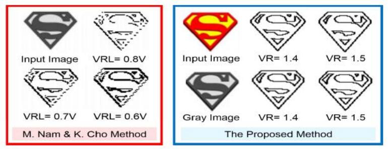
[56]	Nam M, Cho K (2018) Implementation of real-time image edge detector based on a bump circuit and active pixels in a CMOS image sensor. Integration 60: 56–62. doi: 10.1016/j.vlsi.2017.07.005
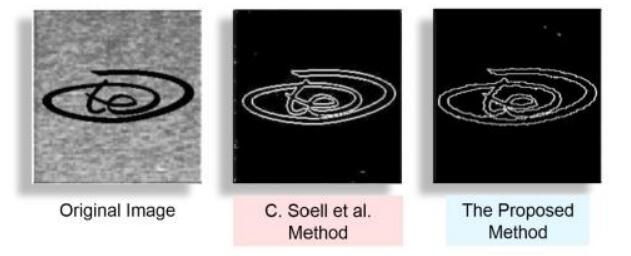
[57]	Soell C, Shi L, Roeber J, et al. (2016) Low-power analog smart camera sensor for edge detection. In: 2016 IEEE International Conference on Image Processing (ICIP), pp. 4408–4412.
[58]	Lee C, Chao W, Lee S, et al. (2015) A Low-Power Edge Detection Image Sensor Based on Parallel Digital Pulse Computation. IEEE Transactions on Circuits and Systems II: Express Briefs 62: 1043–1047. doi: 10.1109/TCSII.2015.2455354
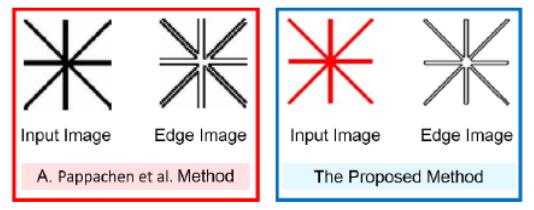
[59]	James A, Pachentavida A, Sugathan S (2014) Edge detection using resistive threshold logic networks with CMOS flash memories. International Journal of Intelligent Computing and Cybernetics 7: 79–94. doi: 10.1108/IJICC-06-2013-0032

This article has been cited by:

1.	Tomislav Došlić, Fusene chains revisited: how kinky they are and why it matters, 2024, 62, 0259-9791, 1595, 10.1007/s10910-024-01620-w
2.	Bai Chunsong, Maham Khalil, Asima Razzaque, Salma Kanwal, Robina Nazir, Saima Noor, Exploring structural variations and topological descriptors of square-hexagonal kink chains of type T2,2 in engineering applications, 2024, 16, 1687-8132, 10.1177/16878132241290418
3.	Saylé Sigarreta, Hugo Cruz-Suárez, Zagreb connection indices on polyomino chains and random polyomino chains, 2024, 22, 2391-5455, 10.1515/math-2024-0057
4.	Shamaila Yousaf, Zaffar Iqbal, Saira Tariq, Adnan Aslam, Fairouz Tchier, Abudulai Issa, Computation of expected values of some connectivity based topological descriptors of random cyclooctane chains, 2024, 14, 2045-2322, 10.1038/s41598-024-57175-y
5.	Xuemin Ling, Asima Razzaque, Maham Khalil, Salma Kanwal, Saima Noor, Robina Nazir, Analysis of expected value of connectivity indices of random 2T2 kink chains, 2025, 13, 2296-424X, 10.3389/fphy.2025.1538443
6.	Kevin Ita, Pegah Capaul, Pardis Khani, Predicting Skin Permeability of Compounds with Elasticnet, Ridge and Decision Tree Regression Methods, 2025, 20, 1872-5120, 10.1007/s12247-025-10025-4

Reader Comments

Your name:*

Email:*
© 2019 the Author(s), licensee AIMS Press. This is an open access article distributed under the terms of the Creative Commons Attribution License (http://creativecommons.org/licenses/by/4.0)