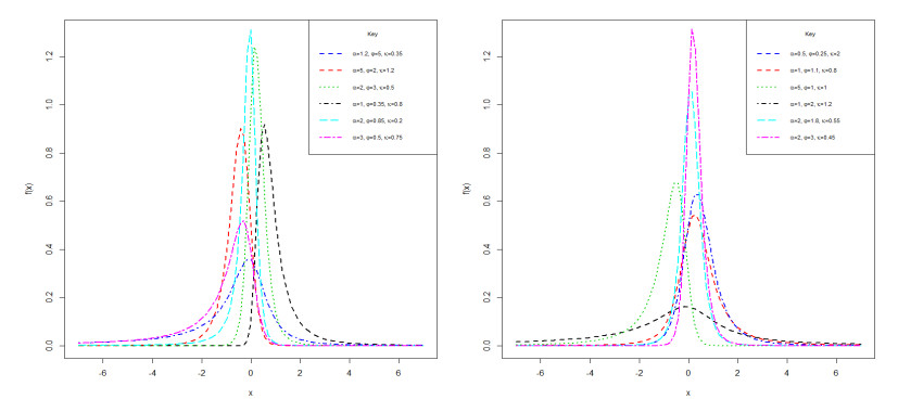
In this work, estimating the exponentiated half logistic skew-t model parameters using some classical estimation procedures is considered. The finite sample performance of the EHLST parameter estimates is examined through extensive Monte Carlo simulations. The ordering performance of the six criterions was based on the partial and overall ranks of the estimation procedures for all parameter combinations. The criterions performance ordering from finest to poorest, using the overall ranks is maximum likelihood, maximum product of spacing, Anderson-Darling, Cramer-von Mises, least squares and weighted least squares estimators for all the parameter combinations. The simulation results confirm the dominance of the maximum likelihood estimation method over other methods with the least overall rank but shows that the maximum product of spacing is most advantageous when the sample size is 200. More so, the EHLST model efficacy is demonstrated through its application on Nigeria inflation rates dataset using the maximum likelihood and maximum product of spacing estimation procedures. Furthermore, the volatility modeling of the Nigeria inflation log-returns using the GARCH-type models with the EHLST innovation density relative to ten commonly used innovation densities validates the superiority of the GARCH (1, 1) and GJRGARCH (1, 1) models with EHLST innovation density in both in-sample and out-samples performance over other models.
Citation: Obinna D. Adubisi, Ahmed Abdulkadir, Chidi. E. Adubisi. A new hybrid form of the skew-t distribution: estimation methods comparison via Monte Carlo simulation and GARCH model application[J]. Data Science in Finance and Economics, 2022, 2(2): 54-79. doi: 10.3934/DSFE.2022003
In this work, estimating the exponentiated half logistic skew-t model parameters using some classical estimation procedures is considered. The finite sample performance of the EHLST parameter estimates is examined through extensive Monte Carlo simulations. The ordering performance of the six criterions was based on the partial and overall ranks of the estimation procedures for all parameter combinations. The criterions performance ordering from finest to poorest, using the overall ranks is maximum likelihood, maximum product of spacing, Anderson-Darling, Cramer-von Mises, least squares and weighted least squares estimators for all the parameter combinations. The simulation results confirm the dominance of the maximum likelihood estimation method over other methods with the least overall rank but shows that the maximum product of spacing is most advantageous when the sample size is 200. More so, the EHLST model efficacy is demonstrated through its application on Nigeria inflation rates dataset using the maximum likelihood and maximum product of spacing estimation procedures. Furthermore, the volatility modeling of the Nigeria inflation log-returns using the GARCH-type models with the EHLST innovation density relative to ten commonly used innovation densities validates the superiority of the GARCH (1, 1) and GJRGARCH (1, 1) models with EHLST innovation density in both in-sample and out-samples performance over other models.

| [1] |
Aas K, Haff IH (2006) The Generalised Hyperbolic Skew Student's t-distribution. J Financ Econ 4: 275-309. https://doi.org/10.1093/jjfinec/nbj006 doi: 10.1093/jjfinec/nbj006

|
| [2] |
Adubisi OD, Abdulkadir A, Chiroma H (2021a) A Two Parameter Odd Exponentiated Skew-t Distribution with J-Shaped Hazard Rate Function. J Stat Model Anal 3: 26-46. https://doi.org/10.22452/josma.vol3no1.3 doi: 10.22452/josma.vol3no1.3
|
| [3] |
Adubisi OD, Abdulkadir A, Chiroma H, et al. (2021b) The Type I Half Logistic Skew-t Distribution: A Heavy-Tail Model with Inverted Bathtub Shaped Hazard Rate. Asian J Probab Stat 14: 21-40. https://doi.org/10.9734/AJPAS/2021/v14i430336 doi: 10.9734/AJPAS/2021/v14i430336
|
| [4] | Adubisi OD, Abdulkadir A, Farouk UA, et al. (2021c) Financial data and a new generalization of the skew-t distribution. Covenant J Phys Life Sci 9: 1-18. |
| [5] |
Aldahlan MAD, Afify AM (2020) The odd exponential half-logistic exponential distribution: Estimation methods and application to Engineering data. Mathematics 8: 1684. https://doi.org/10.3390/math8101684 doi: 10.3390/math8101684
|
| [6] |
Altun E, (2019) Two-sided exponential-geometric distribution: Inference and volatility modeling. Comput Stat 34: 1215-1245. https://doi.org/10.1007/s00180-019-00873-3 doi: 10.1007/s00180-019-00873-3
|
| [7] |
Altun E, Tatlidil H, Ozel G, et al. (2018) A new generalized of skew-T distribution with volatility models. J Stat Comput Simu 88: 1252-1272. https://doi.org/10.1080/00949655.2018.1427240 doi: 10.1080/00949655.2018.1427240
|
| [8] |
Alzaatreh A, Lee C, Famoye F (2013) A new method for generating families of continuous distributions. Metron 71: 63-79. https://doi.org/10.1007/s40300-013-0007-y doi: 10.1007/s40300-013-0007-y
|
| [9] |
Azzalini A, Capitanio A (2003) Distributions generated by perturbation of symmetry with emphasis on a multivariate skew-t distribution. J Roy Statist Soc B 65: 367-389. https://doi.org/10.1111/1467-9868.00391 doi: 10.1111/1467-9868.00391
|
| [10] |
Bakouch HS, Dey S, Ramos PL, et al. (2017) Binomial-exponential 2 distribution: Different estimation methods with weather applications. TEMA 18: 233-251. https://doi.org/10.5540/tema.2017.018.02.0233 doi: 10.5540/tema.2017.018.02.0233
|
| [11] |
Basalamah D, Ning W, Gupta A (2018) The beta skew-t distribution and its properties. J Stat Theory Pract 12: 837-860. https://doi.org/10.1080/15598608.2018.1481468 doi: 10.1080/15598608.2018.1481468
|
| [12] |
Bollerslev T (1986) Generalized Autoregressive Conditional Heteroskedasticity. J Econometrics 31: 307-327. https://doi.org/10.1016/0304-4076(86)90063-1 doi: 10.1016/0304-4076(86)90063-1
|
| [13] |
Brooks C, Burke SP (2003) Information criteria for GARCH model selection. Eur J Financ 9: 557-580. https://doi.org/10.1080/1351847021000029188 doi: 10.1080/1351847021000029188
|
| [14] | Cheng R, Amin N (1979) Maximum product of spacing estimation with application to Lognormal distribution. Mathematical Report 79-1, University of Wales, Cardiff, UK. |
| [15] |
Cheng R, Amin N (1983) Estimating parameters in continuous univariate distributions with a shifted origin. J R Stat Soc Ser B Methodol 45: 394-403. https://doi.org/10.1111/j.2517-6161.1983.tb01268.x doi: 10.1111/j.2517-6161.1983.tb01268.x
|
| [16] |
Chesneau C, Bakouch HS, Ramos PL, et al. (2020) The polynomial-exponential distribution: a continuous probability model allowing for occurrence of zero values. Commun Stat Simul Comput 20: 1-26. https://doi.org/10.1080/03610918.2020.1746339 doi: 10.1080/03610918.2020.1746339
|
| [17] |
Cordeiro GM, Alizadeh M, Ortega EMM (2014) The Exponentiated Half-Logistic Family of Distributions: Properties and Applications. J Probab Stat 21 https://doi.org/10.1155/2014/864396 doi: 10.1155/2014/864396
|
| [18] | Dikko HG, Agboola S (2017) Exponentiated generalized Skew-t distribution. J Nigerian Assoc Math Phys 42: 219-228. |
| [19] |
Engle RF (1982) Autoregressive Conditional Heteroskedasticity with Estimates of the Variance of United Kingdom Inflation. Econometrica 50: 987-1008. https://doi.org/10.2307/1912773 doi: 10.2307/1912773
|
| [20] |
Glosten LR, Jagannathan R, Runkle DE (1993) On the Relation between the Expected Value and the Volatility of the Nominal Excess Return on Stocks. J Financ 48: 1779-1801. https://doi.org/10.1111/j.1540-6261.1993.tb05128.x doi: 10.1111/j.1540-6261.1993.tb05128.x
|
| [21] | Johnson NL, Kotz S, Balakrishnan N (1995) Continuous Univariate Distributions. New York: Wiley. |
| [22] | Jones MC (2001) A skew t distribution. In Probability and Statistical Models with Applications. London: Chapman and Hall, 269-277. |
| [23] |
Jones MC, Faddy MJ (2003) A skew extension of the t-distribution, with applications. J Roy Statist Soc Ser B 65: 159-174. https://doi.org/10.1111/1467-9868.00378 doi: 10.1111/1467-9868.00378
|
| [24] | Khamis KS, Basalamah D, Ning W, et al. (2017) The Kumaraswamy Skew-t Distribution and Its Related Properties. Commun Stat Simul Comput. https://doi.org/10.1080/03610918.2017.1346801. |
| [25] | Louzada F, Ramos PL, Perdoná GS (2016) Different estimation procedures for the parameters of the extended exponential geometric distribution for medical data. Comput Math Methods Med https://doi.org/10.1155/2016/8727951 |
| [26] |
Ramos PL, Louzada F, Ramos E, et al. (2020) The Fréchet distribution: Estimation and application-An overview. J Stat Manage Syst 23: 549-578. https://doi.org/10.1080/09720510.2019.1645400 doi: 10.1080/09720510.2019.1645400
|
| [27] |
Rodrigues GC, Louzada F, Ramos PL (2018) Poisson-exponential distribution: different methods of estimation. J Appl Stat 45: 128-144. https://doi.org/10.1080/02664763.2016.1268571 doi: 10.1080/02664763.2016.1268571
|
| [28] |
Sahu SK, Dey DK, Branco MD (2003) A new class of multivariate skew distributions with applications to Bayesian regression models. Can J Stat 31: 129-150. https://doi.org/10.2307/3316064 doi: 10.2307/3316064
|
| [29] |
Shafiei S, Doostparast M (2014) Balakrishnan skew-t distribution and associated statistical characteristics. Comm Statist Theory Methods 43: 4109-4122. https://doi.org/10.1080/03610926.2012.701697 doi: 10.1080/03610926.2012.701697
|
| [30] | Shittu OI, Adepoju KA, Adeniji OE (2014) On the Beta Skew-t distribution in modelling stock return in Nigeria. Int J Mod Math Sci 11: 94-102. |
| [31] |
ZeinEldin RA, Chesneau C, Jamal F, et al. (2019) Different estimation methods for type I half-logistic Topp-Leone distribution Mathematics 7: 985. https://doi.org/10.3390/math7100985 doi: 10.3390/math7100985
|
 DSFE-02-02-003-s001.pdf DSFE-02-02-003-s001.pdf |
 |


Figures(4) / Tables(13)
Obinna D. Adubisi, Ahmed Abdulkadir, Chidi. E. Adubisi. A new hybrid form of the skew-t distribution: estimation methods comparison via Monte Carlo simulation and GARCH model application[J]. Data Science in Finance and Economics, 2022, 2(2): 54-79. doi: 10.3934/DSFE.2022003


 DownLoad: