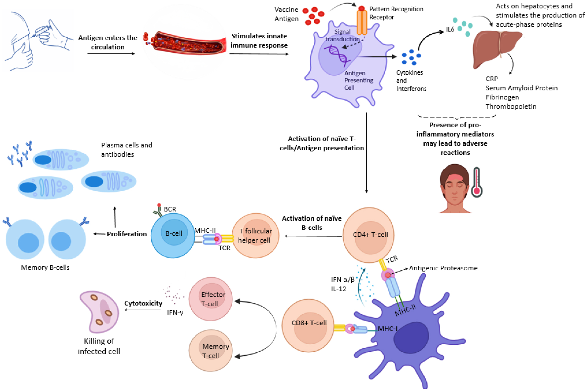
Since the initiation of immunization against SARS-CoV-2, the adverse reactions of vaccines have remained a major contributor to vaccine hesitancy. Their occurrence has been attributed to the immune response against the administered antigen, which is affected by different factors including the age of the vaccine recipient. The trends of the adverse reactions of COVID-19 vaccines have shown a higher frequency in younger adults (18–64 years old) than in the older population (≥65 years). One of the potential reasons is the healthy and efficient immune systems of younger individuals, which provide a robust pro-inflammatory response upon antigen encounter. Their adaptive immune system has a diverse array of naïve T and B lymphocytes, which aids in antigen elimination with the development of a long-lasting immunological memory. Age-related changes in the immune system of the elderly are referred to as immunosenescence, which reduces its efficiency. The phenomenon of cellular senescence and inflammageing can lower the vaccine responses of older recipients. Thymic involution and ageing of the bone marrow can lead to decreased levels of naïve T-cells and memory B-cells. This could compromise the ability to either fight new infections or effectively respond to vaccines and develop a lasting immune memory. Along with clinical trials of senolytic drugs, lifestyle interventions are being studied to mitigate such age-related changes. Further insights into vaccine responses in the elderly population and the means to alleviate the hallmarks of immunosenescence are required.
Citation: Laiba Noor, Syeda Momna Ishtiaq, Farhat Batool, Muhammad Imran Arshad. Age-dependent trends in adverse reactions of SARS-CoV-2 vaccines: A narrative review[J]. AIMS Allergy and Immunology, 2024, 8(3): 146-166. doi: 10.3934/Allergy.2024008
Since the initiation of immunization against SARS-CoV-2, the adverse reactions of vaccines have remained a major contributor to vaccine hesitancy. Their occurrence has been attributed to the immune response against the administered antigen, which is affected by different factors including the age of the vaccine recipient. The trends of the adverse reactions of COVID-19 vaccines have shown a higher frequency in younger adults (18–64 years old) than in the older population (≥65 years). One of the potential reasons is the healthy and efficient immune systems of younger individuals, which provide a robust pro-inflammatory response upon antigen encounter. Their adaptive immune system has a diverse array of naïve T and B lymphocytes, which aids in antigen elimination with the development of a long-lasting immunological memory. Age-related changes in the immune system of the elderly are referred to as immunosenescence, which reduces its efficiency. The phenomenon of cellular senescence and inflammageing can lower the vaccine responses of older recipients. Thymic involution and ageing of the bone marrow can lead to decreased levels of naïve T-cells and memory B-cells. This could compromise the ability to either fight new infections or effectively respond to vaccines and develop a lasting immune memory. Along with clinical trials of senolytic drugs, lifestyle interventions are being studied to mitigate such age-related changes. Further insights into vaccine responses in the elderly population and the means to alleviate the hallmarks of immunosenescence are required.

| [1] |
Abdul-Fattah S, Pal A, Kaka N, et al. (2021) History and recent advances in coronavirus discovery. In Silico Modeling of Drugs Against Coronaviruses . Berlin: Springer 3-24. https://doi.org/10.1007/7653_2020_47 
|
| [2] |
Li YD, Chi WY, Su JH, et al. (2020) Coronavirus vaccine development: From SARS and MERS to COVID-19. J Biomed Sci 27: 104. https://doi.org/10.1186/s12929-020-00695-2
|
| [3] | Umakanthan S, Sahu P, Ranade A V, et al. (2020) Origin, transmission, diagnosis and management of coronavirus disease 2019 (COVID-19). Postgrad Med J 96: 753-758. https://doi.org/10.1136/postgradmedj-2020-138234 |
| [4] |
Dong E, Du H, Gardner L (2020) An interactive web-based dashboard to track COVID-19 in real time. Lancet Infect Dis 20: 533-534. https://doi.org/10.1016/S1473-3099(20)30120-1
|
| [5] |
Matsumura T, Takano T, Takahashi Y (2023) Immune responses related to the immunogenicity and reactogenicity of COVID-19 mRNA vaccines. Int Immunol 35: 213-220. https://doi.org/10.1093/intimm/dxac064
|
| [6] |
Zheng C, Shao W, Chen X, et al. (2022) Real-world effectiveness of COVID-19 vaccines: A literature review and meta-analysis. Int J Infect Dis 114: 252-260. https://doi.org/10.1016/j.ijid.2021.11.009
|
| [7] |
Wise J (2023) Covid-19: WHO declares end of global health emergency. BMJ 381: 1041. https://doi.org/10.1136/bmj.p1041
|
| [8] |
Matrajt L, Eaton J, Leung T, et al. (2021) Vaccine optimization for COVID-19: Who to vaccinate first?. Sci Adv 7: eabf1374. https://doi.org/10.1126/sciadv.abf1374
|
| [9] | Ruiz Estrada MA (2021) The COVID-19 natural selection by age. SSRN Electron J . https://doi.org/10.2139/ssrn.3773704 |
| [10] | Azwar MK, Setiati S, Rizka A, et al. (2020) Clinical profile of elderly patients with COVID-19 hospitalised in Indonesia's national general hospital. Acta Med Indones 52: 199-205. |
| [11] |
Witkowski JM, Fulop T, Bryl E (2022) Immunosenescence and COVID-19. Mech Ageing Dev 204: 111672. https://doi.org/10.1016/j.mad.2022.111672
|
| [12] |
Wang J, Tong Y, Li D, et al. (2021) The impact of age difference on the efficacy and safety of COVID-19 vaccines: A systematic review and meta-analysis. Front Immunol 12: 758294. https://doi.org/10.3389/fimmu.2021.758294
|
| [13] |
Hervé C, Laupèze B, Del Giudice G, et al. (2019) The how's and what's of vaccine reactogenicity. Npj Vaccines 4: 39. https://doi.org/10.1038/s41541-019-0132-6
|
| [14] |
Sprent J, King C (2021) COVID-19 vaccine side effects: The positives about feeling bad. Sci Immunol 6: 1-4. https://doi.org/10.1126/sciimmunol.abj9256
|
| [15] |
Sutton N, San Francisco Ramos A, Beales E, et al. (2022) Comparing reactogenicity of COVID-19 vaccines: A systematic review and meta-analysis. Expert Rev Vaccines 21: 1301-1318. https://doi.org/10.1080/14760584.2022.2098719
|
| [16] |
Palanica A, Jeon J (2022) Initial mix-and-match COVID-19 vaccination perceptions, concerns, and side effects across Canadians. Vaccines 10: 93. https://doi.org/10.3390/vaccines10010093
|
| [17] |
Atyabi SMH, Rommasi F, Ramezani MH, et al. (2022) Relationship between blood clots and COVID-19 vaccines: A literature review. Open Life Sci 17: 401-415. https://doi.org/10.1515/biol-2022-0035
|
| [18] |
Dhamanti I, Suwantika AA, Adlia A, et al. (2023) Adverse reactions of COVID-19 vaccines: A scoping review of observational studies. Int J Gen Med 16: 609-618. https://doi.org/10.2147/IJGM.S400458
|
| [19] |
Segni MT, Demissie HF, Adem MK, et al. (2022) Post COVID-19 vaccination side effects and associated factors among vaccinated health care providers in Oromia region, Ethiopia in 2021. PLoS One 17: e0278334. https://doi.org/10.1371/journal.pone.0278334
|
| [20] |
Villanueva P, McDonald E, Croda J, et al. (2024) Factors influencing adverse events following COVID-19 vaccination. Hum Vaccin Immunother 20. https://doi.org/10.1080/21645515.2024.2323853
|
| [21] |
Abbaspour S, Robbins GK, Blumenthal KG, et al. (2022) Identifying modifiable predictors of COVID-19 vaccine side effects: A machine learning approach. Vaccines 10: 1747. https://doi.org/10.3390/vaccines10101747
|
| [22] |
George A, Goble HM, Garlapati S, et al. (2023) Demographic and lifestyle factors associated with patient-reported acute COVID-19 vaccine reactivity. Vaccines 11: 1072. https://doi.org/10.3390/vaccines11061072
|
| [23] |
Tran VN, Nguyen HA, Le TTA, et al. (2021) Factors influencing adverse events following immunization with AZD1222 in Vietnamese adults during first half of 2021. Vaccine 39: 6485-6491. https://doi.org/10.1016/j.vaccine.2021.09.060
|
| [24] |
Mori M, Yokoyama A, Shichida A, et al. (2023) Impact of sex and age on vaccine-related side effects and their progression after booster mRNA COVID-19 vaccine. Sci Rep 13: 19328. https://doi.org/10.1038/s41598-023-46823-4
|
| [25] |
Gonzalez-Dias P, Lee EK, Sorgi S, et al. (2020) Methods for predicting vaccine immunogenicity and reactogenicity. Hum Vaccin Immunother 16: 269-276. https://doi.org/10.1080/21645515.2019.1697110
|
| [26] |
Zhuang CL, Lin ZJ, Bi ZF, et al. (2021) Inflammation-related adverse reactions following vaccination potentially indicate a stronger immune response. Emerg Microbes Infect 10: 365-375. https://doi.org/10.1080/22221751.2021.1891002
|
| [27] |
Pollard AJ, Bijker EM (2021) A guide to vaccinology: from basic principles to new developments. Nat Rev Immunol 21: 83-100. https://doi.org/10.1038/s41577-020-00479-7
|
| [28] |
Li D, Wu M (2021) Pattern recognition receptors in health and diseases. Signal Transduction Targeted Ther 6: 291. https://doi.org/10.1038/s41392-021-00687-0
|
| [29] |
Lacagnina MJ, Watkins LR, Grace PM (2018) Toll-like receptors and their role in persistent pain. Pharmacol Ther 184: 145-158. https://doi.org/10.1038/s41392-021-00687-0
|
| [30] |
Primorac D, Vrdoljak K, Brlek P, et al. (2022) Adaptive immune responses and immunity to SARS-CoV-2. Front Immunol 13. https://doi.org/10.3389/fimmu.2022.848582
|
| [31] |
Destexhe E, Prinsen MK, van Schöll I, et al. (2013) Evaluation of C-reactive protein as an inflammatory biomarker in rabbits for vaccine nonclinical safety studies. J Pharmacol Toxicol Methods 68: 367-373. https://doi.org/10.1016/j.vascn.2013.04.003
|
| [32] |
Levy I, Levin EG, Olmer L, et al. (2022) Correlation between adverse events and antibody titers among healthcare workers vaccinated with BNT162b2 mRNA COVID-19 vaccine. Vaccines 10: 1220. https://doi.org/10.3390/vaccines10081220
|
| [33] |
Grifoni A, Weiskopf D, Ramirez SI, et al. (2020) Targets of T cell responses to SARS-CoV-2 coronavirus in humans with COVID-19 disease and unexposed individuals. Cell 181: 1489-1501.e15. https://doi.org/10.1016/j.cell.2020.05.015
|
| [34] |
Sette A, Crotty S (2022) Immunological memory to SARS-CoV-2 infection and COVID-19 vaccines. Immunol Rev 310: 27-46. https://doi.org/10.1111/imr.13089
|
| [35] |
Bugya Z, Prechl J, Szénási T, et al. (2021) Multiple levels of immunological memory and their association with vaccination. Vaccines 9: 174. https://doi.org/10.3390/vaccines9020174
|
| [36] |
Wherry EJ, Barouch DH (2022) T cell immunity to COVID-19 vaccines. Science 377: 821-822. https://doi.org/10.1126/science.add2897
|
| [37] |
Cohen KW, Linderman SL, Moodie Z, et al. (2021) Longitudinal analysis shows durable and broad immune memory after SARS-CoV-2 infection with persisting antibody responses and memory B and T cells. Cell Reports Med 2: 100354. https://doi.org/10.1016/j.xcrm.2021.100354
|
| [38] |
Chen WH, Strych U, Hotez PJ, et al. (2020) The SARS-CoV-2 vaccine pipeline: An overview. Curr Trop Med Reports 7: 61-64. https://doi.org/10.1007/s40475-020-00201-6
|
| [39] |
Ndwandwe D, Wiysonge CS (2021) COVID-19 vaccines. Curr Opin Immunol 71: 111-116. https://doi.org/10.1016/j.coi.2021.07.003
|
| [40] |
Rueda-Fernández M, Melguizo-Rodríguez L, Costela-Ruiz VJ, et al. (2022) The current status of COVID-19 vaccines. A scoping review. Drug Discov Today 27: 103336. https://doi.org/10.1016/j.drudis.2022.08.004
|
| [41] |
Kyriakidis NC, López-Cortés A, González EV, et al. (2021) SARS-CoV-2 vaccines strategies: A comprehensive review of phase 3 candidates. Npj Vaccines 6: 28. https://doi.org/10.1038/s41541-021-00292-w
|
| [42] |
Bok K, Sitar S, Graham BS, et al. (2021) Accelerated COVID-19 vaccine development: Milestones, lessons, and prospects. Immunity 54: 1636-1651. https://doi.org/10.1016/j.immuni.2021.07.017
|
| [43] |
Santi Laurini G, Montanaro N, Broccoli M, et al. (2023) Real-life safety profile of mRNA vaccines for COVID-19: An analysis of VAERS database. Vaccine 41: 2879-2886. https://doi.org/10.1016/j.vaccine.2023.03.054
|
| [44] |
Chapin-Bardales J, Myers T, Gee J, et al. (2021) Reactogenicity within 2 weeks after mRNA COVID-19 vaccines: Findings from the CDC v-safe surveillance system. Vaccine 39: 7066-7073. https://doi.org/10.1016/j.vaccine.2021.10.019
|
| [45] |
Faksova K, Walsh D, Jiang Y, et al. (2024) COVID-19 vaccines and adverse events of special interest: A multinational Global Vaccine Data Network (GVDN) cohort study of 99 million vaccinated individuals. Vaccine 42: 2200-2211. https://doi.org/10.1016/j.vaccine.2024.01.100
|
| [46] | GOV.UKArchive: Information for UK recipients on COVID-19 Vaccine AstraZeneca (Regulation 174) (2023). Available from: https://www.gov.uk/government/publications/regulatory-approval-of-covid-19-vaccine-astrazeneca/information-for-uk-recipients-on-covid-19-vaccine-astrazeneca#possible-side-effects |
| [47] |
Raethke M, van Hunsel F, Thurin NH, et al. (2023) Cohort event monitoring of adverse reactions to COVID-19 vaccines in seven European countries: Pooled results on first dose. Drug Saf 46: 391-404. https://doi.org/10.1007/s40264-023-01281-9
|
| [48] | Johnson & JohnsonJohnson & Johnson updates U.S. COVID-19 vaccine fact sheet (2022). Available from: https://www.jnj.com/media-center/press-releases/johnson-johnson-updates-u-s-covid-19-vaccine-fact-sheet |
| [49] |
Amer SA, Al-Zahrani A, Imam EA, et al. (2024) Exploring the reported adverse effects of COVID-19 vaccines among vaccinated Arab populations: A multi-national survey study. Sci Rep 14: 4785. https://doi.org/10.1038/s41598-024-54886-0
|
| [50] |
Akrami M, Hosamirudsari H, Faraji N, et al. (2023) Sputnik V vaccine-related complications and its impression on inflammatory biomarkers in healthcare providers. Indian J Med Microbiol 43: 79-84. https://doi.org/10.1016/j.ijmmb.2022.10.012
|
| [51] |
Granados Villalpando JM, Romero Tapia S de J, Baeza Flores G del C, et al. (2022) Prevalence and risk factors of adverse effects and allergic reactions after COVID-19 vaccines in a Mexican population: An analytical cross-sectional study. Vaccines 10: 2012. https://doi.org/10.3390/vaccines10122012
|
| [52] |
Hasan SS, Rashid A, Osama S, et al. (2022) Covid-19 vaccine safety and adverse event analysis from Pakistan. Clin Immunol Commun 2: 91-97. https://doi.org/10.1016/j.clicom.2022.05.003
|
| [53] |
Mohebbi A, Eterafi M, Fouladi N, et al. (2023) Adverse effects reported and insights following Sinopharm COVID-19 vaccination. Curr Microbiol 80: 377. https://doi.org/10.1007/s00284-023-03432-8
|
| [54] |
Abu-Halaweh S, Alqassieh R, Suleiman A, et al. (2021) Qualitative assessment of early adverse effects of Pfizer–BioNTech and Sinopharm COVID-19 vaccines by telephone interviews. Vaccines 9: 950. https://doi.org/10.3390/vaccines9090950
|
| [55] |
Lai FTT, Leung MTY, Chan EWW, et al. (2022) Self-reported reactogenicity of CoronaVac (Sinovac) compared with Comirnaty (Pfizer-BioNTech): A prospective cohort study with intensive monitoring. Vaccine 40: 1390-1396. https://doi.org/10.1016/j.vaccine.2022.01.062
|
| [56] |
Smith K, Hegazy K, Cai MR, et al. (2023) Safety of the NVX-CoV2373 COVID-19 vaccine in randomized placebo-controlled clinical trials. Vaccine 41: 3930-3936. https://doi.org/10.1016/j.vaccine.2023.05.016
|
| [57] |
Xiong X, Yuan J, Li M, et al. (2021) Age and gender disparities in adverse events following COVID-19 vaccination: Real-world evidence based on big data for risk management. Front Med 8: 700014. https://doi.org/10.3389/fmed.2021.700014
|
| [58] |
Elnaem MH, Mohd Taufek NH, Ab Rahman NS, et al. (2021) COVID-19 vaccination attitudes, perceptions, and side effect experiences in Malaysia: Do age, gender, and vaccine type matter?. Vaccines 9: 1156. https://doi.org/10.3390/vaccines9101156
|
| [59] | UPMC Health BeatHow age and sex couid affect COVID vaccine side effects (2021). Available from: https://share.upmc.com/2021/04/age-and-sex-covid-19-vaccine/ |
| [60] |
Sultana A, Shahriar S, Tahsin MR, et al. (2021) A retrospective cross-sectional study assessing self-reported adverse events following immunization (AEFI) of the COVID-19 vaccine in Bangladesh. Vaccines 9: 1090. https://doi.org/10.3390/vaccines9101090
|
| [61] |
Saeed BQ, Al-Shahrabi R, Alhaj SS, et al. (2021) Side effects and perceptions following Sinopharm COVID-19 vaccination. Int J Infect Dis 111: 219-226. https://doi.org/10.1016/j.ijid.2021.08.013
|
| [62] |
Enayatrad M, Mahdavi S, Aliyari R, et al. (2023) Reactogenicity within the first week after Sinopharm, Sputnik V, AZD1222, and COVIran Barekat vaccines: Findings from the Iranian active vaccine surveillance system. BMC Infect Dis 23: 150. https://doi.org/10.1186/s12879-023-08103-4
|
| [63] | Pagotto V, Ferloni A, Soriano MM, et al. (2021) Active surveillance of the Sputnik V vaccine in health workers. medRxiv : 2021.02.03.21251071. https://doi.org/10.1101/2021.02.03.21251071 |
| [64] |
Weintraub ES, Oster ME, Klein NP (2022) Myocarditis or pericarditis following mRNA COVID-19 vaccination. JAMA Netw Open 5: e2218512. https://doi.org/10.1001/jamanetworkopen.2022.18512
|
| [65] |
Buchan SA, Seo CY, Johnson C, et al. (2022) Epidemiology of myocarditis and pericarditis following mRNA vaccination by vaccine product, schedule, and interdose interval among adolescents and adults in ontario, Canada. JAMA Netw Open 5: e2218505. https://doi.org/10.1001/jamanetworkopen.2022.18505
|
| [66] |
Wise J (2021) Covid-19: European countries suspend use of Oxford-AstraZeneca vaccine after reports of blood clots. BMJ 372: n699. https://doi.org/10.1136/bmj.n699
|
| [67] |
Ghorbani H, Rouhi T, Vosough Z, et al. (2022) Drug-induced hepatitis after Sinopharm COVID-19 vaccination: A case study of a 62-year-old patient. Int J Surg Case Rep 93: 106926. https://doi.org/10.1016/j.ijscr.2022.106926
|
| [68] |
Bril F, Al Diffalha S, Dean M, et al. (2021) Autoimmune hepatitis developing after coronavirus disease 2019 (COVID-19) vaccine: Causality or casualty?. J Hepatol 75: 222-224. https://doi.org/10.1016/j.jhep.2021.04.003
|
| [69] |
Clayton-Chubb D, Schneider D, Freeman E, et al. (2021) Autoimmune hepatitis developing after the ChAdOx1 nCoV-19 (Oxford-AstraZeneca) vaccine. J Hepatol 75: 1249-1250. https://doi.org/10.1016/j.jhep.2021.06.014
|
| [70] |
Beatty AL, Peyser ND, Butcher XE, et al. (2021) Analysis of COVID-19 vaccine type and adverse effects following vaccination. JAMA Netw Open 4: e2140364. https://doi.org/10.1001/jamanetworkopen.2021.40364
|
| [71] |
Oh SJ, Lee JK, Shin OS (2019) Aging and the immune system: The impact of immunosenescence on viral infection, immunity and vaccine immunogenicity. Immune Netw 19: e37. https://doi.org/10.4110/in.2019.19.e37
|
| [72] |
Ciocca M, Zaffina S, Fernandez Salinas A, et al. (2021) Evolution of human memory B cells from childhood to old age. Front Immunol 12: 690534. https://doi.org/10.3389/fimmu.2021.690534
|
| [73] |
Collier DA, Ferreira IATM, Kotagiri P, et al. (2021) Age-related immune response heterogeneity to SARS-CoV-2 vaccine BNT162b2. Nature 596: 417-422. https://doi.org/10.1038/s41586-021-03739-1
|
| [74] |
Yousfi M El, Mercier S, Breuillé D, et al. (2005) The inflammatory response to vaccination is altered in the elderly. Mech Ageing Dev 126: 874-881. https://doi.org/10.1016/j.mad.2005.03.008
|
| [75] |
Hajjo R, Sabbah DA, Bardaweel SK, et al. (2021) Shedding the light on post-vaccine myocarditis and pericarditis in COVID-19 and Non-COVID-19 vaccine recipients. Vaccines 9: 1186. https://doi.org/10.3390/vaccines9101186
|
| [76] |
Lazaros G, Klein AL, Hatziantoniou S, et al. (2021) The novel platform of mRNA COVID-19 vaccines and myocarditis: Clues into the potential underlying mechanism. Vaccine 39: 4925-4927. https://doi.org/10.1016/j.vaccine.2021.07.016
|
| [77] |
Bozkurt B, Kamat I, Hotez PJ (2021) Myocarditis with COVID-19 mRNA vaccines. Circulation 144: 471-484. https://doi.org/10.1161/CIRCULATIONAHA.121.056135
|
| [78] |
Klok FA, Pai M, Huisman MV, et al. (2022) Vaccine-induced immune thrombotic thrombocytopenia. Lancet Haematol 9: e73-e80. https://doi.org/10.1016/S2352-3026(21)00306-9
|
| [79] |
Afshar ZM, Barary M, Babazadeh A, et al. (2022) SARS-CoV-2-related and Covid-19 vaccine-induced thromboembolic events: A comparative review. Rev Med Virol 32: e2327. https://doi.org/10.1002/rmv.2327
|
| [80] |
Mani A, Ojha V (2022) Thromboembolism after COVID-19 vaccination: A systematic review of such events in 286 patients. Ann Vasc Surg 84: 12-20.e1. https://doi.org/10.1016/j.avsg.2022.05.001
|
| [81] |
Avci E, Abasiyanik F (2021) Autoimmune hepatitis after SARS-CoV-2 vaccine: New-onset or flare-up?. J Autoimmun 125: 102745. https://doi.org/10.1016/j.jaut.2021.102745
|
| [82] |
Palla P, Vergadis C, Sakellariou S, et al. (2022) Letter to the editor: Autoimmune hepatitis after COVID-19 vaccination: A rare adverse effect?. Hepatology 75: 489-490. https://doi.org/10.1002/hep.32156
|
| [83] |
Vuille-Lessard É, Montani M, Bosch J, et al. (2021) Autoimmune hepatitis triggered by SARS-CoV-2 vaccination. J Autoimmun 123: 102710. https://doi.org/10.1016/j.jaut.2021.102710
|
| [84] |
Efe C, Kulkarni AV, Terziroli Beretta-Piccoli B, et al. (2022) Liver injury after SARS-CoV-2 vaccination: Features of immune-mediated hepatitis, role of corticosteroid therapy and outcome. Hepatology 76: 1576-1586. https://doi.org/10.1002/hep.32572
|
| [85] |
Torjesen I (2021) Covid-19: Doctors in Norway told to assess severely frail patients for vaccination. BMJ 372: n167. https://doi.org/10.1136/bmj.n167
|
| [86] |
Edler C, Klein A, Schröder AS, et al. (2021) Deaths associated with newly launched SARS-CoV-2 vaccination (Comirnaty®). Leg Med 51: 101895. https://doi.org/10.1016/j.legalmed.2021.101895
|
| [87] |
Torjesen I (2021) Covid-19: Norway investigates 23 deaths in frail elderly patients after vaccination. BMJ 372: n149. https://doi.org/10.1136/bmj.n149
|
| [88] |
Lee KA, Flores RR, Jang IH, et al. (2022) Immune senescence, immunosenescence and aging. Front Aging 3: 900028. https://doi.org/10.3389/fragi.2022.900028
|
| [89] |
Huang W, Hickson LJ, Eirin A, et al. (2022) Cellular senescence: The good, the bad and the unknown. Nat Rev Nephrol 18: 611-627. https://doi.org/10.1038/s41581-022-00601-z
|
| [90] |
Katuuk DA, Lengkong JSJ, Rotty VNJ, et al. (2021) Management of Covid-19 vaccination for the elderly. BIRCI J 4: 2121-2134. https://doi.org/10.33258/birci.v4i2.1902 2121
|
| [91] |
Agrawal A, Weinberger B (2022) Editorial: The impact of immunosenescence and senescence of immune cells on responses to infection and vaccination. Front Aging 3: 882494. https://doi.org/10.3389/fragi.2022.882494
|
| [92] |
Guidi N, Marka G, Sakk V, et al. (2021) An aged bone marrow niche restrains rejuvenated hematopoietic stem cells. Stem Cells 39: 1101-1106. https://doi.org/10.1002/stem.3372
|
| [93] |
de Mol J, Kuiper J, Tsiantoulas D, et al. (2021) The dynamics of B cell aging in health and disease. Front Immunol 12: 733566. https://doi.org/10.3389/fimmu.2021.733566
|
| [94] | Saridena A, Saridena A, Kethar J (2023) Reactions to SARS-CoV-2: The effectiveness of the body's immunological memory. J Student Res 12. https://doi.org/10.47611/jsrhs.v12i1.4359 |
| [95] | Shittu A Understanding immunological memory (2023). Available from: https://asm.org/Articles/2023/May/Understanding-Immunological-Memory |
| [96] |
Condotta SA, Richer MJ (2017) The immune battlefield: The impact of inflammatory cytokines on CD8+ T-cell immunity. PLOS Pathog 13: e1006618. https://doi.org/10.1371/journal.ppat.1006618
|
| [97] |
Wakui M, Uwamino Y, Yatabe Y, et al. (2022) Assessing anti-SARS-CoV-2 cellular immunity in 571 vaccines by using an IFN-γ release assay. Eur J Immunol 52: 1961-1971. https://doi.org/10.1002/eji.202249794
|
| [98] |
Lee HG, Cho MJ, Choi JM (2020) Bystander CD4+ T cells: Crossroads between innate and adaptive immunity. Exp Mol Med 52: 1255-1263. https://doi.org/10.1038/s12276-020-00486-7
|
| [99] |
Martinez-Sanchez ME, Huerta L, Alvarez-Buylla ER, et al. (2018) Role of cytokine combinations on CD4+ T cell differentiation, partial polarization, and plasticity: Continuous network modeling approach. Front Physiol 9: 877. https://doi.org/10.3389/fphys.2018.00877
|
| [100] |
Kedzierska K, Thomas PG (2022) Count on us: T cells in SARS-CoV-2 infection and vaccination. Cell Reports Med 3: 100562. https://doi.org/10.1016/j.xcrm.2022.100562
|
| [101] |
Hall V, Foulkes S, Insalata F, et al. (2022) Protection against SARS-CoV-2 after Covid-19 vaccination and previous infection. N Engl J Med 386: 1207-1220. https://doi.org/10.1056/NEJMoa2118691
|
| [102] |
Yoshida M, Kobashi Y, Kawamura T, et al. (2023) Association of systemic adverse reaction patterns with long-term dynamics of humoral and cellular immunity after coronavirus disease 2019 third vaccination. Sci Rep 13: 9264. https://doi.org/10.1038/s41598-023-36429-1
|
| [103] |
Kobashi Y, Shimazu Y, Kawamura T, et al. (2022) Factors associated with anti-severe acute respiratory syndrome coronavirus 2 (SARS-CoV-2) spike protein antibody titer and neutralizing activity among healthcare workers following vaccination with the BNT162b2 vaccine. PLoS One 17: e0269917. https://doi.org/10.1371/journal.pone.0269917
|
| [104] |
Naaber P, Tserel L, Kangro K, et al. (2021) Dynamics of antibody response to BNT162b2 vaccine after six months: a longitudinal prospective study. Lancet Reg Heal Eur 10: 100208. https://doi.org/10.1016/j.lanepe.2021.100208
|
| [105] |
Koike R, Sawahata M, Nakamura Y, et al. (2022) Systemic adverse effects induced by the BNT162b2 vaccine are associated with higher antibody titers from 3 to 6 months after vaccination. Vaccines 10: 451. https://doi.org/10.3390/vaccines10030451
|
| [106] |
Chi WY, Li YD, Huang HC, et al. (2022) COVID-19 vaccine update: Vaccine effectiveness, SARS-CoV-2 variants, boosters, adverse effects, and immune correlates of protection. J Biomed Sci 29: 82. https://doi.org/10.1186/s12929-022-00853-8
|
| [107] |
Klingel H, Krüttgen A, Imöhl M, et al. (2023) Humoral immune response to SARS-CoV-2 mRNA vaccines is associated with choice of vaccine and systemic adverse reactions DMD TNR. Clin Exp Vaccine Res 12: 60-69. https://doi.org/10.7774/cevr.2023.12.1.60
|
| [108] |
Hwang YH, Song KH, Choi Y, et al. (2021) Can reactogenicity predict immunogenicity after COVID-19 vaccination?. Korean J Intern Med 36: 1486-1491. https://doi.org/10.3904/kjim.2021.210
|
| [109] |
Bauernfeind S, Salzberger B, Hitzenbichler F, et al. (2021) Association between reactogenicity and immunogenicity after vaccination with BNT162b2. Vaccines 9: 1089. https://doi.org/10.3390/vaccines9101089
|
| [110] |
Lim SY, Kim JY, Park S, et al. (2021) Correlation between reactogenicity and immunogenicity after the ChAdOx1 nCoV-19 and BNT162b2 mRNA vaccination. Immune Netw 21: e41. https://doi.org/10.4110/in.2021.21.e41
|
| [111] |
Liu Z, Liang Q, Ren Y, et al. (2023) Immunosenescence: Molecular mechanisms and diseases. Signal Transducttion Targeted Ther 8: 200. https://doi.org/10.1038/s41392-023-01451-2
|
| [112] |
Accardi G, Caruso C (2018) Immune-inflammatory responses in the elderly: An update. Immun Ageing 15: 11. https://doi.org/10.1186/s12979-018-0117-8
|
| [113] |
Thomas R, Wang W, Su DM (2020) Contributions of age-related thymic involution to immunosenescence and inflammaging. Immun Ageing 17: 2. https://doi.org/10.1186/s12979-018-0117-8
|
| [114] | Thomas R, Su DM (2020) Age-related thymic atrophy: Mechanisms and outcomes. Thymus . Vienna: IntechOpen. https://doi.org/10.5772/intechopen.86412 |
| [115] |
Frasca D, Diaz A, Romero M, et al. (2020) B cell immunosenescence. Annu Rev Cell Dev Biol 36: 551-574. https://doi.org/10.1146/annurev-cellbio-011620-034148
|
| [116] |
Slamanig SA, Nolte MA (2021) The bone marrow as sanctuary for plasma cells and memory T-cells: Implications for adaptive immunity and vaccinology. Cells 10: 1508. https://doi.org/10.3390/cells10061508
|
| [117] | Bowdish D, Loukov D, Naidoo A (2015) Immunosenescence: Implications for vaccination programs in the elderly. Vaccine Dev Ther 17. https://doi.org/10.2147/VDT.S63888 |
| [118] |
Connor KM, Hsu Y, Aggarwal PK, et al. (2018) Understanding metabolic changes in aging bone marrow. Exp Hematol Oncol 7: 13. https://doi.org/10.1186/s40164-018-0105-x
|
| [119] |
Bajaj V, Gadi N, Spihlman AP, et al. (2021) Aging, immunity, and COVID-19: How age influences the host immune response to coronavirus infections?. Front Physiol 11: 571416. https://doi.org/10.3389/fphys.2020.571416
|
| [120] |
Cox LS, Bellantuono I, Lord JM, et al. (2020) Tackling immunosenescence to improve COVID-19 outcomes and vaccine response in older adults. Lancet Heal Longev 1: e55-e57. https://doi.org/10.1016/S2666-7568(20)30011-8
|
| [121] | Bardasi EM, Garcia G, Twigg J Covid-19 has exposed the fragilities of aging countries (2021). Available from: https://ieg.worldbankgroup.org/blog/covid-19-has-exposed-fragilities-aging-countries |
| [122] |
Goronzy JJ, Weyand CM (2013) Understanding immunosenescence to improve responses to vaccines. Nat Immunol 14: 428-436. https://doi.org/10.1038/ni.2588
|
| [123] |
Chaib S, Tchkonia T, Kirkland JL (2022) Cellular senescence and senolytics: The path to the clinic. Nat Med 28: 1556-1568. https://doi.org/10.1038/s41591-022-01923-y
|
| [124] |
Zimmermann P, Curtis N (2019) Factors that influence the immune response to vaccination. Clin Microbiol Rev 32. https://doi.org/10.1128/cmr.00084-18
|
| [125] |
Weyh C, Krüger K, Strasser B (2020) Physical activity and diet shape the immune system during aging. Nutrients 12: 622. https://doi.org/10.3390/nu12030622
|
| [126] |
Tylutka A, Morawin B, Gramacki A, et al. (2021) Lifestyle exercise attenuates immunosenescence; flow cytometry analysis. BMC Geriatr 21: 200. https://doi.org/10.1186/s12877-021-02128-7
|
| [127] |
Bencivenga L, Rengo G, Varricchi G (2020) Elderly at time of COronaVIrus disease 2019 (COVID-19): Possible role of immunosenescence and malnutrition. GeroScience 42: 1089-1092. https://doi.org/10.1007/s11357-020-00218-9
|
| [128] |
Lefebvre JS, Haynes L (2013) Vaccine strategies to enhance immune responses in the aged. Curr Opin Immunol 25: 523-528. https://doi.org/10.1016/j.coi.2013.05.014
|


Figures(3) / Tables(1)

Laiba Noor, Syeda Momna Ishtiaq, Farhat Batool, Muhammad Imran Arshad. Age-dependent trends in adverse reactions of SARS-CoV-2 vaccines: A narrative review[J]. AIMS Allergy and Immunology, 2024, 8(3): 146-166. doi: 10.3934/Allergy.2024008


 DownLoad: