Dynamic analysis and optimal control of co-infection system under different outbreak times of mutant strains

Bolin Zhu; Dong Qiu; Bolin Zhu; Dong Qiu

doi:10.3934/Allergy.2024009

AIMS Allergy and Immunology

2024, Volume 8, Issue 3: 167-192. doi: 10.3934/Allergy.2024009

Previous Article Next Article

Research article

Dynamic analysis and optimal control of co-infection system under different outbreak times of mutant strains

Bolin Zhu ,
Dong Qiu ^,

College of Science, Chongqing University of Posts and Telecommunications, Nanan, Chongqing, 400065, China

Received: 16 May 2024 Revised: 01 September 2024 Accepted: 19 September 2024 Published: 29 September 2024

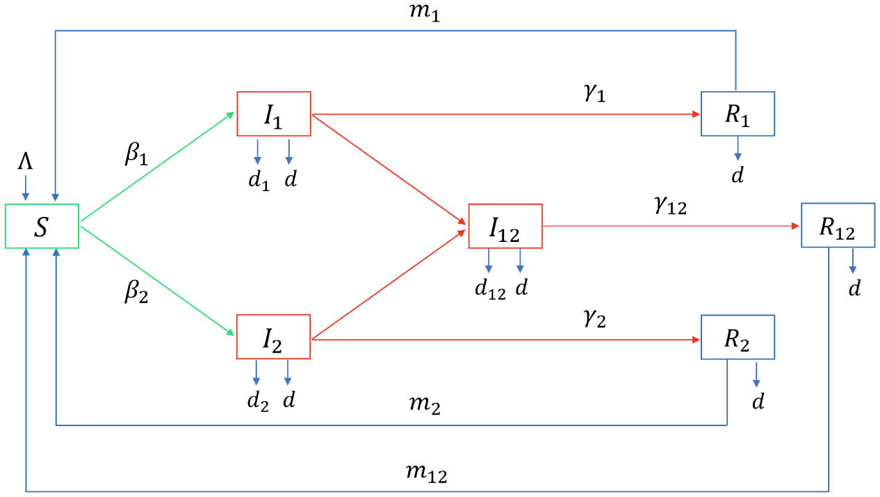
In epidemic prevention efforts, the emergence of new virus strains due to mutations greatly complicates the prediction and management of epidemics. Most of the current mathematical models of infectious diseases assume that the mutant strain and the original strain have the same outbreak time, which is obviously an ideal situation. In order to make the study more practical, we consider the general situation of outbreaks of mutated strains. At the same time, the optimal control strategy under different emergence time of mutant strains was proposed by using the optimal control theory and numerical simulation. This study provides a new theoretical framework for the dual strain competition model with different outbreak times. The final theoretical results and numerical simulation showed that although the emergence time of the mutant did not affect the final trend of the epidemic, it would affect the cost of prevention and control during the control period.
- virus mutation models,
- Lyapunov equation,
- basic reproduction number,
- optimal control,
- Pontryagin's maximum principle
Citation: Bolin Zhu, Dong Qiu. Dynamic analysis and optimal control of co-infection system under different outbreak times of mutant strains[J]. AIMS Allergy and Immunology, 2024, 8(3): 167-192. doi: 10.3934/Allergy.2024009

Related Papers:

Abstract

In epidemic prevention efforts, the emergence of new virus strains due to mutations greatly complicates the prediction and management of epidemics. Most of the current mathematical models of infectious diseases assume that the mutant strain and the original strain have the same outbreak time, which is obviously an ideal situation. In order to make the study more practical, we consider the general situation of outbreaks of mutated strains. At the same time, the optimal control strategy under different emergence time of mutant strains was proposed by using the optimal control theory and numerical simulation. This study provides a new theoretical framework for the dual strain competition model with different outbreak times. The final theoretical results and numerical simulation showed that although the emergence time of the mutant did not affect the final trend of the epidemic, it would affect the cost of prevention and control during the control period.

Acknowledgments

This work was supported by the National Natural Science Foundation of China (Grant Nos. 12171065, 11671001 and 72171031).

Conflict of interest

The authors declare there are no conflicts of interest.

References

[1]	Ismahene Y (2021) Infectious diseases, trade, and economic growth: A panel analysis of developed and developing countries. J Knowl Econ 13: 2547-2583. https://doi.org/10.1007/s13132-021-00811-z
[2]	Morley JE (2021) 2020: The year of the COVID-19 pandemic. J Nutr Health Aging 25: 1-4. https://doi.org/10.1007/s12603-020-1545-7
[3]	He H, Ou Z, Yu D (2022) Spatial and temporal trends in HIV/AIDS burden among worldwide regions from 1990 to 2019: A secondary analysis of the global burden of disease study 2019. Front Med 9. https://doi.org/10.3389/fmed.2022.808318
[4]	Vaux S, Fonteneau L, Pefau M (2023) Vaccination against influenza, measles, pertussis and varicella in workers in healthcare facilities in France: A national cross-sectional study in 2019. Vaccine 41: 812-820. https://doi.org/10.1016/j.vaccine.2022.12.023
[5]	Sweileh WM (2022) Global research activity on mathematical modeling of transmission and control of 23 selected infectious disease outbreak. Glob Health 18: 4. https://doi.org/10.1186/s12992-022-00803-x
[6]	Garira W, Maregere B (2023) The transmission mechanism theory of disease dynamics: Its aims, assumptions and limitations. Infect Dis Model 8: 122-144. https://doi.org/10.1016/j.idm.2022.12.001
[7]	Dietz K, Heesterbeek JAP (2002) Daniel Bernoulli's epidemiological model revisited. Math Biosci 180: 1-21. https://doi.org/10.1016/S0025-5564(02)00122-0
[8]	McQuade ST, Weightman R, Merrill NJ (2021) Control of COVID-19 outbreak using an extended SEIR model. Math Mod Meth Appl S 31: 2399-2424. https://doi.org/10.1142/S0218202521500512
[9]	Wang Z, Bauch CT, Bhattacharyya S (2016) Statistical physics of vaccination. Phys Rep 664: 1-113. https://doi.org/10.1016/j.physrep.2016.10.006
[10]	Chen J, Xia C, Perc M (2024) The SIQRS propagation model with quarantine on simplicial complexes. IEEE Trans Comput Social Syst 1–12. https://doi.org/10.1109/TCSS.2024.3351173
[11]	Nistal R, Sen MDL, Alonso-Quesada S (2015) On the stability and equilibrium points of multistaged SI (n) R epidemic models. Discrete Dyn Nat Soc . https://doi.org/10.1155/2015/379576
[12]	Liu Q, Jiang D, Hayat T (2019) Dynamics of a stochastic multigroup SIQR epidemic model with standard incidence rates. J Franklin Inst 356: 2960-2993. https://doi.org/10.1016/j.jfranklin.2019.01.038
[13]	Nuo M, Castillo-Chavez C, Feng Z (2008) Mathematical models of influenza: The role of cross-immunity, quarantine and age-structure. Mathematical Epidemiology. Berlin, Heidelberg: Springer 349-364. https://doi.org/10.1007/978-3-540-78911-6_13
[14]	Bala S, Gimba B (2019) Global sensitivity analysis to study the impacts of bed-nets, drug treatment, and their efficacies on a two-strain malaria model. Math Comput Appl 24: 32. https://doi.org/10.3390/mca24010032
[15]	Wu Y, Zhang Z, Song L (2024) Global stability analysis of two strains epidemic model with imperfect vaccination and immunity waning in a complex network. Chaos Solitons Fractals 179. https://doi.org/10.1016/j.chaos.2023.114414
[16]	Chen J, Feng M, Zhao D (2023) Composite effective degree Markov chain for epidemic dynamics on higher-order networks. IEEE Trans Syst Man Cybern 53: 7415-7426. https://doi.org/10.1109/TSMC.2023.3298019
[17]	Islam S, Islam T, Islam MR (2022) New coronavirus variants are creating more challenges to global healthcare system: A brief report on the current knowledge. Clin Pathol 15: 1-7. https://doi.org/10.1177/2632010X221075584
[18]	Tchoumi SY, Diagne ML, Rwezaura H (2021) Malaria and COVID-19 co-dynamics: A mathematical model and optimal control. Appl Math Model 99: 294-327. https://doi.org/10.1016/j.apm.2021.06.016
[19]	Brandal LT, MacDonald E, Veneti L (2021) Outbreak caused by the SARS-CoV-2 Omicron variant in Norway. Eurosurveillance 26. https://doi.org/10.2807/1560-7917.ES.2021.26.50.2101147
[20]	Visca D, Ong CWM, Tiberi S (2021) Tuberculosis and COVID-19 interaction: A review of biological, clinical and public health effects. Pulmonology 27: 151-165. https://doi.org/10.1016/j.pulmoe.2020.12.012
[21]	Alene KA, Wangdi K, Clements ACA (2020) Impact of the COVID-19 Pandemic on Tuberculosis Control: An Overview. Trop Med Infect Dis 5: 123. https://doi.org/10.3390/tropicalmed5030123
[22]	Jagannathan P, Wang TT (2021) Immunity after SARS-CoV-2 infections. Nat Immunol 22: 539-540. https://doi.org/10.1038/s41590-021-00923-3
[23]	Beitari S, Duque D, Bavananthasivam J (2023) Cross protection to SARS-CoV-2 variants in hamsters with naturally-acquired immunity. Virol J 20: 167. https://doi.org/10.1186/s12985-023-02136-6
[24]	Song H, Jia Z, Jin Z (2021) Estimation of COVID-19 outbreak size in Harbin, China. Nonlinear Dyn 106: 1229-1237. https://doi.org/10.1007/s11071-021-06406-2
[25]	Lakshmikantham V, Leela S, Martynyuk AA (2015) Stability analysis of nonlinear systems. Switzerland: Springer. https://doi.org/10.1007/978-3-319-27200-9
[26]	Van den Driessche P, Watmough J (2002) Reproduction numbers and sub-threshold endemic equilibria for compartmental models of disease transmission. Math Biosci 180: 29-48. https://doi.org/10.1016/S0025-5564(02)00108-6
[27]	Lasalle J The stability of dynamical systems, Regional Conference Series in Applied Mathematics (1976). https://epubs.siam.org/doi/book/10.1137/1.9781611970432
[28]	Rouche N, Habets P, Laloy M (1977) Stability Theory by Liapunov's Direct Method, Applied Mathematical Sciences. New York: Springer. https://doi.org/10.1007/978-1-4684-9362-7
[29]	Castillo-Chavez C, Song B (2004) Dynamical models of tuberculosis and their applications. Math Biosci Eng 1: 361-404. https://doi.org/10.3934/mbe.2004.1.361
[30]	Mekonen KG, Obsu LL, Habtemichael TG (2022) Optimal control analysis for the coinfection of COVID-19 and TB. Arab J Basic Appl Sci 29: 175-192. https://doi.org/10.1080/25765299.2022.2085445
[31]	Sharomi O, Podder CN, Gumel AB (2007) Role of incidence function in vaccine-induced backward bifurcation in some HIV models. Math Biosci 210: 436-463. https://doi.org/10.1016/j.mbs.2007.05.012
[32]	Gumel AB, Iboi EA, Ngonghala CN (2020) Mathematical assessment of the roles of vaccination and non-pharmaceutical interventions on COVID-19 dynamics: a multigroup modeling approach. Math Biosci 325: 108364. https://doi.org/10.1016/j.mbs.2020.108364
[33]	Ojo MM, Peter OJ, Goufo EFD (2023) A mathematical model for the co-dynamics of COVID-19 and tuberculosis. Math Comput Simul 207: 499-520. https://doi.org/10.1016/j.matcom.2023.01.014
[34]	Goudiaby M, Gning L, Diagne M (2022) Optimal control analysis of a COVID-19 and tuberculosis co-dynamics model. Inform Med Unlocked 28. https://doi.org/10.1016/j.imu.2022.100849
[35]	Agusto F, Numfor E, Srinivasa K (2023) Impact of public sentiments on the transmission of COVID-19 across a geographical gradient. PeerJ 11: e14736. https://doi.org/10.7717/peerj.14736
[36]	Okuonghae D, Omosigho SE (2011) Analysis of a mathematical model for tuberculosis: What could be done to increase case detection. J Theor Biol 269: 31-45. https://doi.org/10.1016/j.jtbi.2010.09.044
[37]	Diagne M, Rwezaura H, Tchoumi S (2021) A mathematical model of COVID-19 with vaccination and treatment. Comput Math Methods Med . https://doi.org/10.1155/2021/1250129
[38]	Omame A, Abbas M, Onyenegecha CP (2021) A fractional-order model for COVID-19 and tuberculosis co-infection using Atangana-Baleanu derivative. Chaos Solitons Fractals 153: 111486. https://doi.org/10.1016/j.chaos.2021.111486
[39]	David J, Iyaniwura SA, Yuan P Modeling the potential impact of indirect transmission on COVID-19 epidemic (2021). https://doi.org/10.1101/2021.01.28.20181040
[40]	Yusuf T, Benyah F (2012) Optimal control of vaccination and treatment for an SIR epidemiological model. World J Model 8: 194-204.
[41]	Pontryagin L, Boltyanski V, Camkrelidze R (1964) The mathematical theory of optimal process. Can Math Bull 7: 500. https://doi.org/10.1017/S0008439500032112
[42]	Boscain U, Piccoli B (2004) Optimal Syntheses for Control Systems on 2-D Manifolds. Berlin, Heidelberg: Springer.

Reader Comments

Your name:*

Email:*
© 2024 the Author(s), licensee AIMS Press. This is an open access article distributed under the terms of the Creative Commons Attribution License (http://creativecommons.org/licenses/by/4.0)