Mean | Median | Min | Max | Kurtosis | Skewness | St.Dev | |
Monthly data | 31560 | 31822 | 24083 | 37158 | -0.31 | -0.42 | 30.44 |
Quarterly data | 32452 | 32675 | 24760 | 37158 | -0.21 | -0.54 | 30.71 |
Citation: J. Nwando Olayiwola, Melanie Raffoul. Saving Women, Saving Families: An Ecological Approach to Optimizing the Health of Women Refugees with S.M.A.R.T Primary Care[J]. AIMS Public Health, 2016, 3(2): 357-374. doi: 10.3934/publichealth.2016.2.357
[1] | Lamya Lairgi, Rachid Lagtayi, Yassir Lairgi, Abdelmajid Daya, Rabie Elotmani, Ahmed Khouya, Mohammed Touzani . Optimization of tertiary building passive parameters by forecasting energy consumption based on artificial intelligence models and using ANOVA variance analysis method. AIMS Energy, 2023, 11(5): 795-809. doi: 10.3934/energy.2023039 |
[2] | Hassan Shirzeh, Fazel Naghdy, Philip Ciufo, Montserrat Ros . Stochastic energy balancing in substation energy management. AIMS Energy, 2015, 3(4): 810-837. doi: 10.3934/energy.2015.4.810 |
[3] | Emrah Gulay . Forecasting the total electricity production in South Africa: Comparative analysis to improve the predictive modelling accuracy. AIMS Energy, 2019, 7(1): 88-110. doi: 10.3934/energy.2019.1.88 |
[4] | P. A. G. M. Amarasinghe, N. S. Abeygunawardana, T. N. Jayasekara, E. A. J. P. Edirisinghe, S. K. Abeygunawardane . Ensemble models for solar power forecasting—a weather classification approach. AIMS Energy, 2020, 8(2): 252-271. doi: 10.3934/energy.2020.2.252 |
[5] | Diksha Kaur, Tek Tjing Lie, Nirmal K. C. Nair, Brice Vallès . Wind Speed Forecasting Using Hybrid Wavelet Transform—ARMA Techniques. AIMS Energy, 2015, 3(1): 13-24. doi: 10.3934/energy.2015.1.13 |
[6] | Muhammad Farhan Hanif, Muhammad Sabir Naveed, Mohamed Metwaly, Jicang Si, Xiangtao Liu, Jianchun Mi . Advancing solar energy forecasting with modified ANN and light GBM learning algorithms. AIMS Energy, 2024, 12(2): 350-386. doi: 10.3934/energy.2024017 |
[7] | Mohamed Elweddad, Muhammet Güneşer, Ziyodulla Yusupov . Designing an energy management system for household consumptions with an off-grid hybrid power system. AIMS Energy, 2022, 10(4): 801-830. doi: 10.3934/energy.2022036 |
[8] | Harry Ramenah, Philippe Casin, Moustapha Ba, Michel Benne, Camel Tanougast . Accurate determination of parameters relationship for photovoltaic power output by augmented dickey fuller test and engle granger method. AIMS Energy, 2018, 6(1): 19-48. doi: 10.3934/energy.2018.1.19 |
[9] | Bilal Akbar, Khuram Pervez Amber, Anila Kousar, Muhammad Waqar Aslam, Muhammad Anser Bashir, Muhammad Sajid Khan . Data-driven predictive models for daily electricity consumption of academic buildings. AIMS Energy, 2020, 8(5): 783-801. doi: 10.3934/energy.2020.5.783 |
[10] | Gokhan Sahin, W.G.J.H.M. Van Wilfried Sark . Estimation of most optimal azimuthal angles for maximum PV solar efficiency using multivariate adaptive regression splines (MARS). AIMS Energy, 2023, 11(6): 1328-1353. doi: 10.3934/energy.2023060 |
In an effort to deal with long-term uncertainties within the energy sector, more accurate long-term peak electricity demand forecasting methods are made use of in decision making and planning purposes. Inaccurate forecasting may seriously result in poor decision making and bad policies establishment. For instance, the South African government, electricity consumers, producers and industries need accurate forecasts for planning future events to assist in long-term development plans for the country in order to minimise risks. The long-term electricity demand forecasting methods are dependent on the choice of variable selections and very importantly, assumptions made for the long run. Researchers have dealt with long-term electricity demand forecasting using different models. For example; Optimal Forecasting Quantile Regression (OFQR), Multiple Simple Linear Regression (MSLR), Artificial Neutral Networks (ANNs), Quantile Regression (QR) and time series analysis models have been used for long-term electricity demand forecasting ([1,2,3,4,5] and [6] among others).
Short-term electricity demand forecasting has attracted substantial attention than medium and long-term forecasting [3]. However, QRA is a new approach and produces more accurate long-term point forecasts for electricity peak demand. The model also performs well in practice for both short and medium-term peak electricity demand. It also gives the smallest values based on prediction intervals (PIs). This has been confirmed in the following literature; for example, [5,7] and [8] among others.
The popularity of long-term peak electricity demand forecasting is mainly motivated by the need to understand the various uncertainties associated with the decision making processes in the South African industries. According to [9], the development of renewable energy policy activities by the South African government is greatly influenced by factors such as the periodical occurrence of different policy crises as a result of economic instability. The key interest for this study is identifying the linear relationship between the response and predictor variables using GAMs, OLS and QR models. OLS estimates quantify the relationship around the mean of the distribution while QR quantifies the relationship across all the various quantiles. Moreover, QR is robust in handling extreme value points of the response variable. Secondly, the electricity demand in South Africa is higher in winter than in summer and influenced especially by irregular events like extreme weather conditions. Also, generally electricity demand is non-stationary and exhibits an upward trend due to mainly economic and population growth. The long-term electricity demand forecasting is essential to avoid the shortage of electricity that may hamper the South African economic growth. South Africa needs reliable forecasts of electricity demand to mitigate the risk of shortages in the future so as to guarantee sustainability.
Although the short-term electricity demand is most widely applied, the long-term peak electricity demand is increasing in popularity with papers such as those by [4] who estimate long-term peak demand by comparing different techniques using a typical fast growing methodology with dynamic electricity demand characteristics and typical developing methodology. Empirical results show that the model is superior, although it uses single electricity demand observation and is capable of giving several electricity demand peak forecasts corresponding at different levels of maximum temperature and some level of social activities. However, it is not easy to rely on a single methodology for determining the electricity demand of such a fast growing and changing system.
The work done by [3] describes in a comparative manner that electricity demand forecasting is divided into three groups, namely, short, medium and long-term electricity demand forecasting. Long-term electricity demand forecasting normally deals with long time horizons. These include one year to ten years and sometimes up to three decades ahead forecast. Furthermore, it is often characterized by large uncertainties created by these distant horizons.
On modelling and forecasting long-term daily peak electricity demand, applied partially linear additive quantile regression (PLAQR) model is applied by [10] using South African data ranging from January 2007 to December 2013. Some data obtained from the 28 South African weather stations divided into coastal and inland regions are used. Variable selection is carried out using Lasso. The empirical results are presented with a comparative analysis of two developed models namely; with pairwise interactions and without interactions. Based on the pinball loss function, the average loss suffered by PLAQR with pairwise interaction is less than that of PLAQR without interaction. Moreover, based on RMSE, MAE and MAPE, PLAQR with pairwise interaction is better than PLAQR without interaction. The empirical results have also shown the usefulness of PLAQR models.
In recent paper, the proposed approaches such as GAMs, additive quantile regression (AQR) with and without interactions and QRA models are used for short-term probabilistic hourly load forecasting in [8]. The authors consider using average pinball loss function for model comparisons and also constructed PI indices such as prediction interval with nominal confidence (PINC), prediction interval widths (PIWs), prediction interval normalised average widths (PINAWs) and prediction interval normalised average deviations (PINADs) for the comperative evaluation of three different models. In their discussion, they indicated that QRA model gives the superior results as it produces the most accurate forecasts compared to other models. It also produces the smallest PINAW and PINAD values.
The study performed by [11] utilizes QR model for peak load demand forecasting to create the estimates of daily peak load demand. The proposed method is used based on its ability to avoid underprediction of the peak load demand and risk of power blackouts. The empirical results show that constructing the quantile from 0.97 to 0.99 is sufficient to estimate the upper limit for the daily peak demand. The authors proposed that the QR model performances should also be compared in other empirical data (for example, economic and financial data). However, in contrast to our study, the authors did not utilize QRA and GAMs in their analysis. This paper considers QRA approach as a comprehensive forecasting solution for long-term peak electricity demand using monthly and quarterly data.
Considering an overview on electricity demand forecasting in section 1.2, the major contributions of this study are summarised in this manner: (1) the study is concentrated on QRA methodology to forecast long-term electricity demand; (2) the developed method should be useful in producing improved forecasting results; (3) the study could answer many challenges and increase the potential to develop a strategy in generating capacity planning and system reliable assessment of dealing with long-term peak electricity demand in South Africa; (4) the long-term electricity demand forecasting solution is discussed and the best forecasting model for future peak electricity demand suggested and (5) the peak electricity demand literature seems scarce in South Africa on the issue of long-term electricity demand and this closes a gap by introducing new methodology to forecast long-term peak electricity demand.
The study considers monthly and quarterly data for peak electricity demand forecasting using quantile regression methods based on the following arguments. Firstly, the paper evaluates accuracy measures of both OLS and QR models. A comparative analysis is done using generalised additive models. The final structure of the paper is organised as follows: In Section 2, we first present the generalised additive models, followed by quantile regression models and then later explores more on additive quantile regression and quantile regression averaging. In Section 3, we present variable selection methods using cross validation (CV), Least absolute shrinkage and selection operator (Lasso) and elastic net. In Section 4, we briefly summarise the empirical results as well as discussing further the general remarks of the results. The results in this section are found using the statistical package ‘r’. Lastly, in Section 5, we wrap up with the conclusion.
Focusing on the main interest of this paper, we lay out the methodology for fitting the monthly and quarterly peak electricity demand with OLS, GAMs, QR and QRA. Then combine the forecasts using some forecast combination methods.
Generalized additive model (GAM) is developed by [12]. GAM is known to be a simple powerful technique that is easy to interpret, more flexible because the relationships between dependent and independent variables are not assumed to be linear and the regularization of predictor functions assist to avoid overfitting effect [13]. In generalized additive models the response variable is expressed as sum of smooth functions. GAMs capture the common non linear patterns which the linear regression technique fails to do. Let $ y_{t} $ denote hourly peak demand and $ \mu_{t} = E(y_{t}) $, then the model can be written as:
$ g(μt)=xx∗tΘΘ+f1(x1t)+f2(x2t)+f3(x3t,x4t)+…, $ | (2.1) |
where $ \pmb{x}^{\ast}_{t} $ is a row of the model matrix for any strictly parametric model components, $ \pmb{\Theta} $ is the corresponding parameter vector, $ f_{i} $ are smooth functions of the covariates, $ x_{it} $ and $ f_{1}, f_{2}, f_{3}... $ are estimated by maximizing a penalized log-likelihood function analogous to the penalized least squares criterion. The GAMs are built around penalised regression smoothers and one of them is called cubic spline smoother [14]. Cubic splines are smoothest interpolators that minimize the penalized least squares. However, they have many free parameters to be smoothed and this seems to be a wasteful exercise. We usually estimate $ g(x_{t}) $ by minimizing
$ n∑t=1{yt−f(xt)}2+λ∫f″(x)2dx, $ | (2.2) |
where $ \lambda $ is a non-negative smoothing parameter. If $ \lambda $ tends to infinity, the penalty term becomes more important and forces $ f^{''}(x) $ to zero. The bigger the value of $ \lambda $, the more the curves become smoother. In this paper, cubic smoothing splines as a solution to optimization problem is used.
QR was introduced by [15] and is described in detail in [16] as an extension of classical least squares estimation of conditional mean models to conditional quantile function. An updated QR theory captures this method as a particular center of the distribution, minimizing the weighted absolute sum of deviations [17]. The conditional quantile function is given by
$ Qτ(yt|xxt)=xxTtββτ+εt, $ | (2.3) |
where, $ 0 < \tau < 1 $ and $ Q_\tau (y_{t}|\pmb {x}_{t}) $ denotes the conditional function for the $ \tau^{th} $ quantile of the electricity demand. Given a set of training data $ G = (y_{t}, \pmb {x}^{T}_{t})^{T} $ for $ t = 1, ..., G $, the parameter $ \pmb{\beta}_{\tau} $ can be estimated as
$ ˆβˆβτ=argmin1G{τ∑t:yt≥xxTtββτ|yt−xxTtββτ|+(1−τ)∑t:yt<xxTtββτ|yt−xxTtββτ|}. $ | (2.4) |
The parameter $ \pmb{\widehat{\beta}}_{\tau} $ in Eq 2.4 is usually estimated by using linear programming methods called least absolute deviation (LAD) regression. If $ \tau $ = $ 0.5 $, Eq 2.4 is now given by
$ ˆβˆβτ=1GG∑t=1|yt−xxTtββτ|, $ | (2.5) |
giving the Ł1 (median regression) estimator. Eq 2.4 can also be written as
$ ˆβˆβτ=1GG∑t=1ρτ(yt−xxTtββτ)=1GG∑t=1(τ−11yt−xxTtββτ<0)(yt−xxTtββτ), $ | (2.6) |
where $ \rho_{\tau} $ is a check function such that $ \rho_{\tau}(b) = \tau(b) $ if $ b\geq0 $ and $ \rho_{\tau}(b) $ = $ (\tau-1)b $ if $ b < 0 $, $ \pmb{1}_{B} $ is the indicator function of the event B.
The study done by [18] proposes the boosting AQR procedure for forecasting uncertainty using electricity smart meter data. The authors consider boosting procedure to estimate an AQR model for a set of quantiles of the future distribution. According to [18], the $ k^{th} $-step ahead forecast for the condition at $ \tau^{th} $-quantile of the electricity demand in equation (2.3) can be estimated using the pinball loss function defined by
$ L(yt,Qτ)={τ(yt−ˆQτ)ifyt≥ˆQτ;(1−τ)(ˆQτ−yt)ifyt<ˆQτ, $ | (2.7) |
where $ \widehat{Q}_{\tau} $ denotes the quantile forecast and $ y_{t} $ represents the actual value of peak electricity demand.
QRA is another recent forecast combination technique used to compute the prediction interval. Despite its popularity and simplicity, it is noted that combining forecasts has not been performed widely in the area of long-term peak electricity demand forecasting using quarterly or monthly data. However, it has been performing well in the practice of electricity price forecasting (see, [7,19], among others). According to [18] the QRA model is given by
$ yt=gk(xxt)+εt, $ | (2.8) |
where $ \pmb{x}_{t} = (\pmb{y}_{t}, \pmb{z}_{t}) $; $ \pmb{z}_{t} $ is a vector of exogenous variables known at time $ t $; $ \pmb{y}_{t} $ is a vector of past demand occurring prior to time $ t $; $ \varepsilon_{t} $ denotes the model error term with $ E[\varepsilon_{t}] = 0 $ and $ E[\pmb{x}_{t}\varepsilon_{t}] = 0 $.
The following section briefly discusses three variable selection methods for penalised regression which includes Lasso, CV and elastic net. Lasso guarantees both variable selection and shrinkage simultaneously. Unlike other penalised regression techniques, in Lasso some of the coefficients may be shrunken all the way to zero. The Lasso estimates for the OLS regression model is given by
$ ^ββ=argminp∑j=1(yy−xxββj)2+λ1p∑j=1|ββj|, $ | (3.1) |
where, $ \pmb{y} = (\pmb{y}_{1}, ..., \pmb{y}_{n}^{T} $ is the response vector and $ \pmb{x}_{j} = (\pmb{x}_{1j}, ..., \pmb{x}_{nj})^{T}, j = 1, ..., p $ are the linear independent predictor, $ \lambda $ is the Lasso regularization parameter, $ \sum^{p}_{j = 1}|\pmb{\beta}_{j}|\leq t $ is called Lasso penalty and $ t $ is the Lasso turning parameter [20]. If $ p > n $, the Lasso selects at most $ n $ variables. There is however an adaptive Lasso method and this method modifies the Lasso penalty by applying weights to each parameter that forms the Lasso constraint. Elastic net is a regularization and variable selection method suggested by [21]. The method removes the limitation on the number of selected variables and also encourages grouping effect that Lasso fails to do. The elastic net estimator is given by
$ ^ββ=argminp∑j=1(yy−xxββj)2+λ1p∑j=1|ββj|+λ2p∑j=1ββ2j, $ | (3.2) |
where, $ \sum^{p}_{j = 1}|\pmb{\beta}_{j}|\leq t_{1} $ and $ \sum^{p}_{j = 1}\pmb{\beta}^{2}_{j} < t_{2} $ are elastic net penalties, $ t_{1} $ and $ t_{2} $ are elastic net turning parameters. Cross validation is another most commonly used selection criterion method that uses part of the training data set to fit the model and the remaining part estimate the prediction error. The data consist of $ 28 $ South African weather stations divided into interior and coastal regions with monthly and quarterly peak electricity demand (MPED and QPED) data, temperature, lagged demand and calendar effects. The MPED and QPED are used as the dependent variables while temperature, lagged demand and calendar effects are used as predictor variables. For MPED, the temperature effects for coastal are AMTC, maxTC and minTC defined as average monthly coastal, average maximum and minimum coastal temperatures respectively. The effects for interior include AMTI, maxTI and minTI defined as average monthly interior, average maximum and minimum interior temperatures respectively.
Likewise, for QPED the temperature effects for coastal are AQTC, maxTC and minTC defined as average quarterly coastal, average maximum and minimum coastal temperatures respectively. The effects for quarterly interior include AQTI, maxTI and minTI defined as average quarterly interior, average maximum and minimum interior temperatures respectively. The temperature effects for both monthly and quarterly peak electricity demand coastal and interior are given by average minimum of coastal and interior temperatures (AminTCI), average of average coastal and interior temperatures (AATCI), average maximum of coastal and interior temperatures (AmaxTCI), difference between average maximum of coastal and interior temperatures (DmaxTCI), difference between average minimum of coastal and interior temperatures (DminTCI) and the difference between average of average monthly coastal and interior temperatures (DAAMTCI) and the difference between average of average quarterly coastal and interior temperatures (DAAQTCI). Furthermore, day type (day of the week), day before holiday (DBH), day after holiday (DAH) and day holiday (DH) are defined as calender effects.
In forecasting electricity demand at inland and coastal regions, we use long-term peak electricity demand models. The QR models are used for both monthly and quarterly data. This study will explore the inclusion of monthly temperature covariates that will also be included in the peak electricity demand parameters through heating and cooling degree days which can be calculated as:
$ HDDt=max(Tref−Tt,0) $ |
and
$ CDDt=max(Tt−Tref,0). $ |
The total monthly heating degree-days ($ \mbox{MHDD}_t $) and the total monthly cooling degree-days ($ \mbox{MCDD}_t $) are calculated as:
$ MHDDt=max[m∑j=1HDDt,j−m∑j=1CDDt,j,0] $ |
and
$ MCDDt=max[m∑j=1CDDt,j−m∑j=1HDDt,j,0] $ |
which reduces to
$ MHDDt=max[m∑j=1(max(Tref−Tt,j,0))−m∑j=1(max(Tt,j−Tref,0)),0] $ |
and
$ MCDDt=max[m∑j=1(max(Tt,j−Tref,0))−m∑j=1(max(Tref−Tt,j,0)),0], $ |
respectively, where $ m $ is the number of days in month $ t $, $ T_t $ is average daily temperature on day $ t $ and $ T_{\mbox{ref}} $ is the reference temperature which separates cold temperatures from hot temperatures. Based on the description of variable selection given in section 3.1, the following MPED models for electricity demand are proposed:
Model 1:
Linear quantile regression (LQR) without interactions model is given as
$ Qτ(MPED|xxt)=α0+α1(DH)+α2(DAH)+α3(DBH)+α4(Daytype)+α5(CDDAminTCI)+α6(CDDAmaxTCI)+α7(HDDAAMTCI)+α8(HDDAminTCI)+α9(noltrend)+εt,τ, $ | (3.3) |
where $ \alpha_{0}, \alpha_{1}, ..., \alpha_{9} $ are constants, CDDAminTCI and CDDAmaxTCI are cooling degree days average minimum and maximum coastal and interior temperatures, HDDAAMTCI is monthly heating degree days average of average coastal and interior temperature, HDDAminTCI is heating degree days average minimum coastal and interior temperature, noltrend is a non-linear trend, $ \varepsilon_{t, \tau} $ is residual error.
Model 2: LQR with interactions model is given by
$ Qτ(MPED|xxt)=α0+α1(DAH)+α2(DBH)+α3(Daytype)+α4(CDDAminTCI∗Daytype)+α5(CDDAmaxTCI)+α6(HDDAAMTCI)+α7(HDDAminTCI)+α8(noltrend)+εt,τ. $ | (3.4) |
Model 3: QRA is given in Eq 3.5
$ MPED=α0+α1(fOLS)+α2(fGAM)+α3(fQR)+εt,τ, $ | (3.5) |
where fOLS, fGAM and fQR are ordinary least squares, generalised additive model and quantile regression forecasts respectively.
Similarly we can drive the formulae for calculating the total quarterly heating and cooling degree-days $ QHDD_{t} $ and $ QCDD_{t} $ respectively as in the monthly formulae. The quarterly temperature covariate will be included in the long-term peak electricity demand parameters through heating and cooling degree-days. Based on the description of variable selection given in section 3.1, the following QPED models for electricity demand are proposed:
Model 4: LQR without interactions model is given as
$ Qτ(QPED|xxt)=α0+α1(DH)+α2(DAH)+α3(Daytype)+α4(CDDAminTCI)+α5(CDDAmaxTCI)+α6(CDDAAQTCI)+α7(noltrend)+εt,τ, $ | (3.6) |
where HDDAAQTCI is quarterly heating degree days average of average coastal and interior temperature.
Model 5: LQR with interactions model is given as
$ Qτ(QPED|xxt)=α0+α1(DH)+α2(DAH)+α3(Daytype)+α4(CDDAminTCI)+α5(CDDAmaxTCI)+α6(HDDAAQTCI∗Dytype)+α7(noltrend)+εt,τ. $ | (3.7) |
Model 6: QRA is given in equation (3.8)
$ QPED=α0+α1(fOLS)+α2(fGAM)+α3(fQR)+εt,τ. $ | (3.8) |
The QR model defined in Eq 2.3 will be helpful in this analysis. The parameter for OLS over $ \pmb {\beta} $ is estimated by minimizing:
$ n∑t=1r(yt−xxTtββ)=n∑t=1(yt−xxTtββ)2, $ | (3.9) |
where $ r $ is the quadratic loss function and the parameter for MLE over $ \pmb {\beta} $ based on the sample $ \{\pmb {x}_{t}, y_{t}\}_{t = 1}^{n} $ is calculated by maximizing
$ L(β)∝exp{−12σ2n∑t=1(yt−xxTtββ)2}. $ | (3.10) |
Stochastic gradient boosting (SGB) is a modification of Gradient boosting (GB) which is a machine learning technique. It fits an additive model in a stage-wise way. The additive model can take the form given in Eq 3.11 ([22]).
$ f(x)=M∑m=1βmb(x;γm), $ | (3.11) |
where $ b(x; \gamma_m) \in \mathbb{R} $ are functions of $ x $ which are characterised by the expansion parameters $ \gamma_m $, $ \beta_m $. The parameters $ \beta_m $ and $ \gamma_m $ are fitted in a stage-wise way, a process which slows down over-fitting ([22]). With SGB, a random sample of the training data set is taken without replacement. A more detailed discussion of this is found in [23].
Support vector regression (SVR) which is based on support vector machines (SVM) uses different kernel functions which map low dimensional data to high dimensional space. SVR was introduced by [24] and estimates a regression function of the form given in Eq (3.12).
$ f(x)=xTw+b, $ | (3.12) |
where $ b $ is a scalar and $ \omega $ is a vector of weights. Eq (3.12) can be reformulated as a quadratic programming problem (QPP) by introducing an $ \varepsilon $-insensitive loss function as given in Eq (3.13) ([24]).
$ min $ | (3.13) |
where $ C > 0, \varepsilon > 0 $ are input parameters, $ \xi_1 = (\xi_{11}, ..., \xi_{1m})^T $ and $ \xi_2 = (\xi_{21}, ..., \xi_{2m}) $ are slack variables.
In this study, the South African monthly and quarterly electricity demand data from Eskom ranging from January 2000 to March 2014 are used. The agammaegate energy data with 5204 daily observations are used to create 171 monthly and 57 quarterly data for analysis. Both training data (Jan 2000–Dec 2008) and testing (Jan 2009–Mar 2014) are used for MPED and QPED modelling. The temperature data for coastal and interior regions from 28 South African weather stations are considered. The study uses the most common variables that have been included in the electricity demand models which include, average monthly and quarterly electricity demand, non linear trend and temperature.
It further analyses three different benchmark models which are GAMs, SVR and SGB. The use of at least two benchmark models is consistent with current trends in forecasting. Current trends in forecasting use a variety of models, statistical models, including comparative analysis with machine learning models. In this study we use one statistical learning benchmark model which is the generalized additive model and two machine learning models, stochastic gradient boosting and support vector regression. Using at least two benchmark models helps us to see how good our model is against well-known methods which produce accurate forecasts. See for instance, [25].
Figures 1 and 2 show monthly and quarterly peak electricity demand (MPED and QPED) plots for the period 2000 to 2014 with density, q-q and box plots respectively. Both MPED and QPED plots show upward trends with strong seasonality. The presence of increasing trends are indicated by the overall upward drifts in the time series. The seasonal variations produce the regular fluctuations from year to year but appear similar across months and quarters.
Table 1 shows the summary statistics for both monthly and quarterly electricity demand data ranging from 1 January 2000 to 31 March 2014. The minimum and maximum values are compared and also used to asses the spread behaviour of both quarterly and monthly electricity demand. The minimum values of MPED and QPED from January–March 2000 and on Monday, January 2000 are 24083 and 24760 MW respectively. Moreover, the maximum value of both MPED and QPED from April-June 2007 and also on Thursday, 24 May 2007 is 37158 MW. The kurtosis values of MPED and QPED are -0.31 and -0.21 respectively. The values indicate that both MPED and QPED data do not perfectly follow the normal distribution. Furthermore, negative kurtosis shows that the distribution has lighter tails and flatter peaks compared to the normal distribution. Table 1 also reveals that both monthly and quarterly electricity demand data are left skewed.
Tables 2 and 3 present the summary results of OLS forecast and QR, QRA, GAMs forecasts for both MPED and QPED models based on RMSE, MAE and MAPE respectively. In Table 2, M1 and M2 represent OLS forecast without and with interactions, respectively, for MPED model, while M4 and M5 represent OLS forecast without and with interactions, respectively, for QPED model.
Likewise, in Table 3, M1 and M2 represent linear QR forecast without and with interactions, respectively, for MPED model while M4 and M5 represent linear QR forecast without and with interactions, respectively, for QPED model, M3 and M6 are QRA forecast for MPED and QPED model respectively, M7 and M8 are GAMs forecast for both MPED and QPED models. The values of RMSE = 79.95 MW, MAE = 72.45 MW and MAPE = 0.22 MW for M4 in Table 2 are less compared to that of M1, M2 and M5 models. Likewise, the values of RMSE = 76.55 MW, MAE = 51.61 MW and MAPE = 0.16 MW for M6 in Table 3 are less compared to that of M1, M2, M3, M4, M5, M7 and M8 models. Moreover, the values of RMSE, MAE and MAPE for M6 (QRA for QPED) are less compared to that of M4 (OLS for MPED). The results of RMSE, MAE and MAPE for M6 (QRA for QPED) also confirm that the model is doing well compared to that of M3 (QRA for MPED). In addition, the values of RMSE, MAE and MAPE for benchmark (SVR and SGB) models in Table 4 are larger than that of M6 model.
Figures 8 and 10 show the results of cross validation estimates of the mean squared prediction error for ridge, Lasso and elastic net models in dependence on the regularization parameter (log of lamda). The numbers on top of each figures shows the number of non-zero regression coefficients. The mean squared prediction errors suggest the smaller values of the parameter that shrinks the coefficients to optimal. Figures 9 and 11 show the coefficient paths for ridge, Lasso and elastic net model independence on log of lamda for $ \alpha $ = 0, 1 and 0.5 respectively. The analysis was also done repeated using different values of $ \alpha $.
The comparison of MPED cross validation estimates of the mean squared prediction error for ridge, lasso and elastic net in Figure 8 shows that the variable selection method called Lasso is superior compared to other methods. There are also noticeable differences in cross validation estimates for all the methods for which Lasso gives the best estimates. Using Lasso and elastic net regression model for model selection, only one non-zero coefficient shows that the function has chosen the second vertical line on the cross validation. This shows that the model might be doing a good job. In Figure 9, all coefficients of ridge regression model are essentially zero when the log of lamda is 15. However, as we relax lamda, the coefficients moves away from zero in a nice smooth way. In fitting Lasso, a lots of the r squared what are explained as quite heavily shrunk coefficients but towards the end coefficients increases (grow very large). This may suggest that at the end of the path, the model might be overfitted. Furthermore, elastic net regression model looks like Lasso with slight differences and this confirms that it is an extension of Lasso proposed by [20]. However, elastic net does not perform satisfactory because there are two shrinkage procedures such as ridge and Lasso in it. Double shrinkage might introduce unnecessary bias. Likewise, Figure 10 shows the QPED model selection of ridge, Lasso and elastic net where the dotted red lines show the cross validation curve. The two dashed lines in Figure 10 also show log of lambda values that gives the minimum mean square errors for cross validation (left dashed line) and that is within one standard error(right dashed line). Figure 11 shows all coefficients of ridge regression model to be zeros when the value of lambda is 14 or more. It can be seen from figure 11 that Lasso regression shrinks the regression coefficients to zero as lambda increases. For instance, when log of lambda $ = 2 $ there are 6 non zero coefficients and when log of lambda $ = 0 $ all coefficients are zero.
Mean | Median | Min | Max | Kurtosis | Skewness | St.Dev | |
Monthly data | 31560 | 31822 | 24083 | 37158 | -0.31 | -0.42 | 30.44 |
Quarterly data | 32452 | 32675 | 24760 | 37158 | -0.21 | -0.54 | 30.71 |
M1 | M2 | M4 | M5 | |
RMSE | 327.91 | 338.12 | 79.95 | 172.17 |
MAE | 252.06 | 262.83 | 72.45 | 128.41 |
MAPE | 0.77 | 0.80 | 0.22 | 0.37 |
M1 | M2 | M3 | M4 | M5 | M6 | M7 | M8 | |
RMSE | 324.89 | 345.38 | 315.46 | 87.92 | 87.97 | 76.55 | 315.96 | 165.94 |
MAE | 249.31 | 273.41 | 231.70 | 73.55 | 73.64 | 51.61 | 235.01 | 123.57 |
MAPE | 0.76 | 0.83 | 0.71 | 0.22 | 0.22 | 0.16 | 0.72 | 0.36 |
GAMs are considered as simple and powerful technique because they provide more flexible predictor functions that uncover hidden patterns in the data and regularize the predictor functions. Moreover, this is one of the techniques that is mostly indispensable in the analysis of long-term peak electricity demand forecasting. This machine learning technique is considered as one of benchmark models in MPED and QPED analysis.
Model 7: Monthly data model GAM is given as
$ \begin{equation} \begin{split} MPED & = \alpha_{0}+s(Daytype)+\alpha_{1}(DH)+\alpha_{2}(CDDAminTCI)+ \alpha_{3}(CDDAmaxTCI)\\&+ \alpha_{4}(HDDAAMTCI)+\alpha_{5}(HDDAminTCI)+s(noltrend)+\varepsilon_{t,\tau}, \end{split} \end{equation} $ | (4.1) |
Model 8: Quarterly data model GAM is given as
$ \begin{equation} \begin{split} QPED& = \alpha_{0}+\alpha_{1}(DH)+\alpha_{2}(DAH)+ s(Daytype)\\&+\alpha_{3}(CDDAminTCI) +\alpha_{4}(CDDAmaxTCI)+ \alpha_{5}(HDDAAQTCI*Daytype)\\&+s(noltrend)+\varepsilon_{t,\tau}, \end{split} \end{equation} $ | (4.2) |
where $ s $ represents smoothing.
SVR (benchmark) | SGB(benchmark) | |
RMSE | 398.35 | 728.19 |
MAE | 325.73 | 558.98 |
MAPE | 0.98 | 1.66 |
Figures 1 and 2 display monthly and quarterly peak electricity demand plots for the period 2000 to 2014 respectively. Hence, Figure 3 shows monthly and quarterly average temperature plots. It also shows strong seasonal effects. The smallest values of RMSE, MAE and MAPE in OLS forecast model (M4) for both MPED and QPED are 79.95 MW, 72.45 MW and 0.22 MW respectively. Likewise, the smallest RMSE, MAE and MAPE in QRA model (M6) are 76.5 MW, 51.61 MW and 0.16 MW respectively.
Table 4 shows the error levels (RMSE = 398.35 MW, MAE = 325.73 MW, MAPE = 0.98 MW) of SVR to be lower than the error level (RMSE = 728.19 MW, MAE = 558.98 MW, MAPE = 166 MW) of SGB model. Figures 6 and 7 show the SVR and SGB benchmark model forecasts for MPED. Clearly, we can see that SVR forecasts in Figure 6 fit very well compared to SGB forecasts in Figure 7. Figures 4 and 5 show the actuals of both MPED and QPED with quantile regression forecast (fQR), generalised additive model forecast (fGAM) and quantile regression averaging forecast (fQRA) respectively. Figure 5 shows fQRA fits very well in QPED data.
In this study the long-term monthly and quarterly peaks electricity demand forecasting using South African data have been presented and therefore the policies to control the supply of electricity are required to make sure that the electricity demand is met to support the South African community. By using monthly and quarterly data and then later applying QR models, the more precise long-term forecasting models are developed. The QR models are becoming more attractive to long-term electricity demand modelling this days as it enables us to construct new quantile functions easily. We believe this study will make important contribution in all research application areas more especially in short, medium or long-term peak electricity demand methodology. QRA model in QPED has the smallest RMSE, MAE and MAPE compared to other models. The Lasso model gives best estimates compared to other variable selection methods. The empirical results of proposed models are suitable not just for long-term electricity demand forecasting, but also for testing policies geared towards the expansion of the electricity infrastructure that should be intensified in South Africa in order to cope with the increasing demand exercised by the country's economic growth and rapid industrialisation programme. QRA is a new technique and performed well in QPED data for long-term electricity demand and it did not perform bad in MPED data also. However, it is not advisable to rely only on a single approach for determining the electricity demand in such a fast growing and changing system of South African economy.
The authors are grateful to the National Research Foundation of South Africa for funding this research, to Eskom, South Africa's power utility company for providing the data, University of Limpopo for their resources and to the numerous people for helpful comments on this paper.
The authors declare no conflict of interest.
[1] | United Nations. Refugees, the numbers: Resources for Speakers on Global Issues. 2015. Available from: http://www.un.org/en/globalissues/briefingpapers/refugees/. |
[2] | European Commission, Directorate-General for Health and Food Safety. Health assessment of refugees and migrants in the EU/EEA. 2015. Available from: http://ec.europa.eu/dgs/health_food-safety/docs/personal_health_handbook_en.pdf. |
[3] | Frances Nicholson, United Nations High Commission for Refugees. Refugee women, survivors, protectors, providers. 2011. Available online from: http://www.unhcr.org.uk/resources/monthly-updates/november-2011-update/refugee-women-survivors-protectors-providers.html. |
[4] | Fazel M, Reed R, Panter-Brick C, et al. (2012) Mental health of displaced and refugee children resettled in high-income countries: risk and protective factors. Lancet 379, no. 9812: 266-82. |
[5] | Lucas, R. (2005) International migration to the high-income countries: Some consequences for economic development in the sending countries. Are we on track to achieve the Millennium Development Goals: 127-81. |
[6] | United Nations High Commission for Refugees. A new beginning: Refugee integration in Europe. 2013. Available from: www.unhcr.org/52403d389.pdf. |
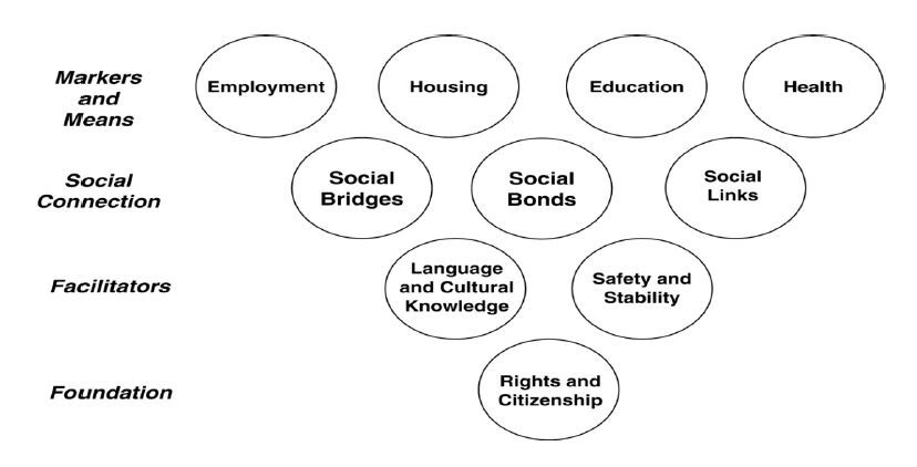
[7] | Ager A, Strang A. (2008) Understanding integration: A conceptual framework. J Refug Stud 21(2): 166-91. |
[8] | Robinson, V. (1998) Defining and measuring successful refugee integration. In Proceedings of ECRE International conference on Integration of Refugees in Europe, Antwerp November 1998. |
[9] | Ager, Alastair, and Alison Strang. Indicators of integration: Final report. Home Office, Research, Development and Statistics Directorate, 2004. |
[10] |
Fazel M, Wheeler J, Danesh J. (2005) Prevalence of serious mental disorder in 7000 refugees resettled in Western countries: A systematic review. Lancet 365:1309-14. doi: 10.1016/S0140-6736(05)61027-6
![]() |
[11] |
Asgary R, Segar M. (2011) Barriers to healthcare access among refugee asylum seekers. J Health Care for the Poor and Underserved 22:506-522. doi: 10.1353/hpu.2011.0047
![]() |
[12] | Pollard R, Betts, W, Carroll J, et al. (2014) Integrating primary care with behavioral health with four special populations: children with special needs, people with serious mental illness, refugees, and deaf people. Am Psychol 69(4): 377-87. |
[13] | Executive board of the United Nations Entity for Gender Equality and the Empowerment of Women. 2011. Available online from: http://www.unwomen.org/~/media/Headquarters/Attachments/Sections/Executive%20Board/EB-2011-AS-UNW-2011-09-StrategicPlan-en.pdf. |
[14] | Women, U. N., and UN Global Compact. "Women’s Empowerment Principles: Equality Means Business." New York City: UN Women, 2010. |
[15] | The Partnership for Maternal, Newborn, and Child health; Partners in Population and development. Women’s empowerment and gender equality: Promoting women’s empowerment for better health outcomes for women and children. 2013. Available online from: http://www.opml.co.uk/sites/default/files/sb_gender_0.pdf. |
[16] | Kishor, S. (2000) Empowerment of women in Egypt and links to the survival and health of their infants. In B.Presser & G. Sen (Eds.), Women’s empowerment and demographic processes. 119-156. New York: Oxford University Press. |
[17] | Kar S, Pascual C, Chickering K. (1999) Empowerment of women for health promotion: a meta-analysis. Soc Sci Med 49(11): 1431-60. |
[18] | Costa, D. (2007). Health care of refugee women. Australian Family Physician 36(3): 151. |
[19] | Starfield B, Shi L, Macinko J. (2005) Contribution of primary care to health systems and health. Milbank Q 83(3): 457-502. |
[20] | World Health Organization. "The World Health Report 2008: Primary health care (now more than ever)." Available online from: http://www.who.int/whr/2008/whr08_en.pdf. |
[21] | Declaration of Alma-Ata, 1978. World Health Organization, 2005. |
[22] | Redwood-Campbell L, Thind H, Howard M, et al. (2008) Understanding the health of refugee women in host countries: lessons from the Kosovar re-settlement in Canada. Prehospital and Disaster Med 23(04): 322-7. |
[23] | Hadle C, Zodhiates A, Sellen D. (2007) Acculturation, economics and food insecurity among refugees resettled in the USA: a case study of West African refugees. Public Health Nutr 10(4): 405-12. |
[24] | Pumariega A, Rothe E, Pumariega J. (2005) Mental health of immigrants and refugees. Community Ment Health J 41(5): 581-97. |
[25] | O'Hare T, Van Tran T. (1998) Substance abuse among Southeast Asians in the US: Implications for practice and research. Soc Work in Health Care 26 (3): 69-80. |
[26] | Wieland M, Weis J, Palmer T, et al. (2012) Physical activity and nutrition among immigrant and refugee women: a community-based participatory research approach. Women's Health 22(2): e225-e232. |
[27] | Hynie M, Crooks V, Barragan J. (2011) Immigrant and refugee social networks: determinants and consequences of social support among women newcomers to Canada. Can J Nurs Res 43(4): 26-46. |
[28] | Lim S. (2009) Loss of Connections Is Death: Transnational Family Ties Among Sudanese Refugee Families Resettling in the United States. J Cross-Cult Psychol 40, no. 6: 1028-40. |
[29] | Muggeridge H, Dona G. (2006) Back Home? Refugees' experiences of their first visit back to their country of origin. J Refug Stud 19(4): 415-32. |
[30] | McPherson, M. (2010) ‘I Integrate, Therefore I Am’: Contesting the Normalizing Discourse of Integrationism through Conversations with Refugee Women. J Refug Stud feq040. |
[31] | Kennedy J, Seymour D, Hummel B. (1999) A comprehensive refugee health screening program. Public Health Rep 114(5): 469. |
[32] | Colic-Peisker V, Walker I. (2003) Human capital, acculturation and social identity: Bosnian refugees in Australia. J Community & Appl Soc Psychol 13, no. 5: 337-60. |
[33] | Oxman-Martinez J, Abdool S. (2000) Immigration, women and health in Canada. Can J Public Health 91(5): 394. |
[34] | Wrigley, H. (2007). Beyond the life boat: Improving language, citizenship and training services for immigrants and refugees. In A. Belzer (Ed.) Toward defining and improving quality in adult basic education: Issues and challenges. Mahwah, New Jersey, Erlbaum Publishing, 221-239. |
[35] | Wolf M, Ly U, Hobart M, Kernic M. (2003) Barriers to seeking police help for intimate partner violence. J Fam Violence 18(2):121-9. |
[36] | United Nations High Commission for Refugees. News stories: New Delhi police teach refugee women how to take care of themselves. 2012. Available from: http://www.unhcr.org/507410439.html. |
[37] | Fong, R. (Ed.). (2004). Culturally competent practice with immigrant and refugee children and families. Guilford Press. |
[38] | Lurie N, Jung M, Lavizzo-Mourey R. (2005) Disparities and quality improvement: federal policy levers. Health Aff 24(2): 354-64. |
[39] | Higgins, Andrew for the New York Times: Norway offers migrants a lesson in how to treat women. 2015. Available from: http://www.nytimes.com/2015/12/20/world/europe/norway-offers-migrants-a-lesson-in-how-to-treat-women.html?_r=1. |
[40] | Olayiwola, Willard-Grace, Dube, Hessler, Shunk, Gottlieb (unpublished data, manuscript under review). |
[41] | Bachrach D, Pfister H, Wallis K, et al. Addressing patients’ social needs: An emerging business case for provider investment. The Commonwealth Fund. 2014. Available from: http://www.commonwealthfund.org/~/media/files/publications/fund-report/2014/may/1749_bachrach_addressing_patients_social_needs_v2.pdf. |
[42] | Tipirneni R, Vickery K, Ehlinger, E. (2015) Accountable Communities for Health: Moving From Providing Accountable Care to Creating Health. Ann Fam Med 13(4): 367-9. |
[43] | Van Dooren G, Coomans S, Struyven L. (2014) Identifying Policy Innovations increasing Labour Market Resilience and Inclusion of Vulnerable Groups National Report Belgium. INSPIRES Working Paper Series 14: 1-48. |
[44] | European Resettlement Network. Belgium Stakeholder Conference on Refugee Resettlement. 2015. Available from: http://www.resettlement.eu/page/belgium-stakeholder-conference-refugee-resettlement-brussels-june-23-2015. |
[45] | San Francisco Department of Public Health. Community health equity and promotion: Newcomers Health Program. Available from: https://www.sfdph.org/dph/comupg/oprograms/CHPP/Newcomers/NewcomersStaffSites.asp. |
[46] | Heather Knight for SF Gate. Medicine S.F. General provides lifeline to traumatized asylum-seekers. 2011. Available from: http://www.sfgate.com/bayarea/article/S-F-General-s-refugee-clinic-a-lifeline-to-care-2366663.php. |
[47] | Theo Chang for the White House blog. Making good use of AARA funding: Frank Kiang Medical Center. 2010. Available from: https://www.whitehouse.gov/blog/2010/08/02/making-good-use-aara-funding-frank-kiang-medical-center. |
[48] | Chang K, Jeung J, Pei P, et al. (2014) "Opening Access for Burmese and Karen Immigrant and Refugee Populations in California: A Blueprint for Integrated Health Service Expansion to Emerging Asian Communities." AAPI Nexus: Policy, Pract Community 12(1-2): 225-44. |
[49] | Chang K, Pei P, Charlemagne L, et al. The Intersection of Culture and Behavioral Health —— Moving Beyond Language. Community Health Forum Magazine. National Association of Community Health Centers. 2012. Available from: http://www.nachc.com/magazine-article.cfm?MagazineArticleID=228. |
[50] |
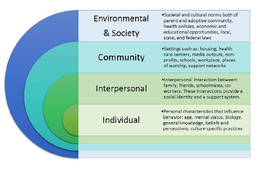
Edberg M, Cleary S, Vyas A. (2011) A trajectory model for understanding and assessing health disparities in Immigrant/Refugee communities. J Immigr Minority Health 13: 576-84.
n Canada. Can J Public Health 91(5): 394. doi: 10.1007/s10903-010-9337-5
![]() |
1. | Luis F.M. Sepulveda, Petterson S. Diniz, João O.B. Diniz, Stelmo M.B. Netto, Carolina L.S. Cipriano, Alexandre C. Araújo, Victor H.B. Lemos, Alexandre C.P. Pessoa, Darlan B.P. Quintanilha, João D.S. Almeida, Aristófanes C. Silva, Anselmo C. Paiva, Geraldo Braz, Márcia I.A. Silva, Eliana M.G. Monteiro, Italo F.S. Silva, Eduardo C. Fernandes, Forecasting of individual electricity consumption using Optimized Gradient Boosting Regression with Modified Particle Swarm Optimization, 2021, 105, 09521976, 104440, 10.1016/j.engappai.2021.104440 |
Mean | Median | Min | Max | Kurtosis | Skewness | St.Dev | |
Monthly data | 31560 | 31822 | 24083 | 37158 | -0.31 | -0.42 | 30.44 |
Quarterly data | 32452 | 32675 | 24760 | 37158 | -0.21 | -0.54 | 30.71 |
M1 | M2 | M4 | M5 | |
RMSE | 327.91 | 338.12 | 79.95 | 172.17 |
MAE | 252.06 | 262.83 | 72.45 | 128.41 |
MAPE | 0.77 | 0.80 | 0.22 | 0.37 |
M1 | M2 | M3 | M4 | M5 | M6 | M7 | M8 | |
RMSE | 324.89 | 345.38 | 315.46 | 87.92 | 87.97 | 76.55 | 315.96 | 165.94 |
MAE | 249.31 | 273.41 | 231.70 | 73.55 | 73.64 | 51.61 | 235.01 | 123.57 |
MAPE | 0.76 | 0.83 | 0.71 | 0.22 | 0.22 | 0.16 | 0.72 | 0.36 |
SVR (benchmark) | SGB(benchmark) | |
RMSE | 398.35 | 728.19 |
MAE | 325.73 | 558.98 |
MAPE | 0.98 | 1.66 |