
Citation: Dreaves Hilary A. How Health Impact Assessments (HIAs) Help Us to Select the Public Health Policies Most Likely to Maximise Health Gain, on the Basis of Best Public Health Science[J]. AIMS Public Health, 2016, 3(2): 235-241. doi: 10.3934/publichealth.2016.2.235
[1] | Hany Bauomy . Safety action over oscillations of a beam excited by moving load via a new active vibration controller. Mathematical Biosciences and Engineering, 2023, 20(3): 5135-5158. doi: 10.3934/mbe.2023238 |
[2] | Hany Bauomy, Ashraf Taha . Nonlinear saturation controller simulation for reducing the high vibrations of a dynamical system. Mathematical Biosciences and Engineering, 2022, 19(4): 3487-3508. doi: 10.3934/mbe.2022161 |
[3] | Xiaoyu Du, Yijun Zhou, Lingzhen Li, Cecilia Persson, Stephen J. Ferguson . The porous cantilever beam as a model for spinal implants: Experimental, analytical and finite element analysis of dynamic properties. Mathematical Biosciences and Engineering, 2023, 20(4): 6273-6293. doi: 10.3934/mbe.2023270 |
[4] | Abdulaziz Alsenafi, M. Ferdows . Effects of thermal slip and chemical reaction on free convective nanofluid from a horizontal plate embedded in a porous media. Mathematical Biosciences and Engineering, 2021, 18(4): 4817-4833. doi: 10.3934/mbe.2021245 |
[5] | Hao Chen, Shengjie Li, Xi Lu, Qiong Zhang, Jixining Zhu, Jiaxin Lu . Research on bearing fault diagnosis based on a multimodal method. Mathematical Biosciences and Engineering, 2024, 21(12): 7688-7706. doi: 10.3934/mbe.2024338 |
[6] | Jagadeesh R. Sonnad, Chetan T. Goudar . Solution of the Michaelis-Menten equation using the decomposition method. Mathematical Biosciences and Engineering, 2009, 6(1): 173-188. doi: 10.3934/mbe.2009.6.173 |
[7] | Ganjun Xu, Ning Dai, Sukun Tian . Principal stress lines based design method of lightweight and low vibration amplitude gear web. Mathematical Biosciences and Engineering, 2021, 18(6): 7060-7075. doi: 10.3934/mbe.2021351 |
[8] | Igor Grigorev, Albert Burgonutdinov, Valentin Makuev, Evgeniy Tikhonov, Viktoria Shvetsova, Oksana Timokhova, Sergey Revyako, Natalia Dmitrieva . The theoretical modeling of the dynamic compaction process of forest soil. Mathematical Biosciences and Engineering, 2022, 19(3): 2935-2949. doi: 10.3934/mbe.2022135 |
[9] | Zulqurnain Sabir, Muhammad Asif Zahoor Raja, Abeer S. Alnahdi, Mdi Begum Jeelani, M. A. Abdelkawy . Numerical investigations of the nonlinear smoke model using the Gudermannian neural networks. Mathematical Biosciences and Engineering, 2022, 19(1): 351-370. doi: 10.3934/mbe.2022018 |
[10] | Anna Andrews, Pezad Doctor, Lasya Gaur, F. Gerald Greil, Tarique Hussain, Qing Zou . Manifold-based denoising for Ferumoxytol-enhanced 3D cardiac cine MRI. Mathematical Biosciences and Engineering, 2024, 21(3): 3695-3712. doi: 10.3934/mbe.2024163 |
Brucellosis is an infectious bacterial disease often spread via direct contact with infected animals or contaminated animal products [1,2]. Brucellosis can transmit to other animals through direct contacts with infected animals or indirect transmission by brucella in the environment. The disease primarily affects cattle, sheep and dogs. In the real world, the infected sheep remain the main source of brucellosis infection, and the basic ewes and other sheep (which includes stock ram and fattening sheep) are often mixed feeding together, therefore there must exist the mixed cross infection between other sheep and basic ewes [3]. Brucellosis is prevalent for more than a century in many parts of the world, and it is well controlled in most developed countries. However, more than 500,000 new cases are reported each year around the world [4,5,6,7].
Mathematical modeling has the potential to analyze the mechanisms of transmission and the complexity of epidemiological characteristics of infectious diseases [8]. In recent years, several mathematical modeling studies have reported on the transmission of brucellosis [3,9,10,11,12,13,14,15,16,17,18,19]. However, these earlier models have mainly focused on the spread of brucellosis between sheep and human through using the dynamic model. Only Li et al [3] proposed a deterministic multi-group model to study the brucellosis transmission among sheep (which the flock of sheep were divided into basic ewes and other sheep). However, they only gave the global stability of disease-free equilibrium and the existence the endemic equilibrium, but the uniqueness and global stability of the endemic equilibrium were not shown when the basic reproduction number is larger than 1. Multi-group model is a class of highly heterogenous models with complex interactions among distinct groups, and the difficulty of global dynamics of multi-group models lies in establishing uniqueness and global stability of endemic equilibrium when basic reproduction number is larger than one [20]. In this paper, we want to study the global dynamic behavior of multi-group type model for the transmission of brucellosis among sheep which are absent from previous papers [3]. We prove the uniqueness of positive endemic equilibrium through using proof by contradiction, and the global stability of endemic equilibrium by using Lyapunov function. Especially, we give the specific coefficients of global Lyapunov function, and show the calculation method of these specific coefficients. By running numerical simulations for the cases with the basic reproduction number to demonstrate the global stability of the equilibria and the unique endemic equilibrium, respectively. By some sensitivity analysis of the basic reproduction number on parameters, we find that vaccination rate of sheep and seropositive detection rate of recessive infected sheep are very important factor for brucellosis.
This paper is organized as follows. In Section 2, we present the dynamical model. And the mathematical analysis including the uniqueness and global stability of positive endemic equilibrium will be given in Section 3. In Section 4, some numerical simulations are given on the global stability of the equilibria and the unique endemic equilibrium. Section 5 gives a discussion about main results.
In previous paper [3], we proposed a multi-group model with cross infection between sheep and human. In this model, $ S_{o}(t), E_{o}(t), I_{o}(t), V_{o}(t) $ and $ S_{f}(t), E_{f}(t), I_{f}(t), V_{f}(t) $ represent susceptible, recessive infected, quarantined seropositive infected, vaccinated other sheep and basic ewes, respectively. $ W(t) $ denotes the quantity of sheep brucella in the environment. $ S_{h}(t), I_{h}(t), Y_{h}(t) $ represent susceptible individuals, acute infections, chronic infections, respectively. There are some assumptions on the dynamical transmission of brucellosis among sheep and from sheep to humans, which are demonstrated in the flowchart (See Figure 1). The following ordinary differential equations can describe a multi-group brucellosis model with Figure 1:
$ {dSodt=Ao−(βooEo+βofEf+βoW)So+λoVo−(γo+do)So,dEodt=(βooEo+βofEf+βoW)So−(co+do)Eo,dIodt=coEo−(αo+do)Io,dVodt=γoSo−(λo+do)Vo,dSfdt=Af−(βffEf+βfoEo+βfW)Sf+λfVf−(γf+df)Sf,dEfdt=(βffEf+βfoEo+βfW)Sf−(cf+df)Ef,dIfdt=cfEf−(αf+df)If,dVfdt=γfSf−(λf+df)Vf,dWdt=ko(Eo+Io)+kf(Ef+If)−(δ+nτ)W,dShdt=Ah−(βhoEo+βhfEf+βhW)Sh−dhSh+pIh,dIhdt=(βhoEo+βhfEf+βhW)Sh−(m+dh+p)Ih,dYhdt=mIh−dhYh. $
|
(2.1) |
Because the last three equations are independent of the first nine equations, we can only consider the first nine equations. Rewrite system (2.1) for general form into the following model:
$ {dSidt=Ai−(di+γi)Si+λiVi−2∑j=1βijSiEj−βiSiW,dEidt=2∑j=1βijSiEj+βiSiW−(di+ci)Ei,dIidt=ciEi−(di+αi)Ii,dVidt=γiSi−(λi+di)Vi,dWdt=2∑i=1ki(Ei+Ii)−δW.i=1,2. $
|
(2.2) |
Adding the first four equations of (2.2) gives
$ \frac{d (S_{i}+E_{i}+I_{i}+V_{i})}{dt}\leq A_{i}-d_{i}(S_{i}+E_{i}+I_{i}+V_{i}), $ |
which implies that $ \lim\limits_{t\rightarrow\infty}\sup(S_{i}+E_{i}+I_{i}+V_{i})\leq\frac{A_{i}}{d_{i}} $. It follows from the last equation of (2.2) that $ \lim\limits_{t\rightarrow\infty}\sup W\leq \frac{\sum^{2}\limits_{i = 1}\frac{k_{i}A_{i}}{d_{i}}}{\delta} $. Hence, the feasible region
$ X = \{(S_{1},E_{1},I_{1},V_{1},S_{2},E_{2},I_{2},V_{2},W)| 0\leq S_{i}+E_{i}+I_{i}+V_{i}\leq\frac{A_{i}}{d_{i}},0\leq W \leq \frac{\sum^{2}\limits_{i = 1}\frac{k_{i}A_{i}}{d_{i}}}{\delta},i = 1,2.\} $ |
is positively invariant with respect to model (2.2). Model (2.2) always admits the disease-free equilibrium $ P_{0} = (S_{i}^{0}, 0, 0, V_{i}^{0}, 0)i = 1, 2 $ in $ X $, where $ S_{i}^{0} = \frac{A_{i}(\lambda_{i}+d_{i})}{d_{i}(d_{i}+\lambda_{i}+\gamma_{i})}, V_{i}^{0} = \frac{A_{i}\gamma_{i}}{d_{i}(d_{i}+\lambda_{i}+\gamma_{i})} $, and $ P_{0} $ is the unique equilibrium that lies on the boundary of $ X $.
According to the definition of $ \mathcal{R}_{c} $ in [21,22,23] and the calculation of $ \mathcal{R}_{o} $ in our previous paper [3], we can obtain the basic reproduction number of model (2.2) is
$ \mathcal{R}_{0} = \rho(FV^{-1}) = \frac{A_{11}+A_{22}+\sqrt{(A_{11}-A_{22})^{2}+4A_{12}A_{21}}}{2}, $ |
where
$ A_{11} = \frac{S_{1}^{0}}{d_{1}+c_{1}}(\beta_{11}+\frac{\beta_{1}k_{1}(d_{1}+\alpha_{1}+c_{1})}{\delta(d_{1}+\alpha_{1})}), A_{12} = \frac{S_{1}^{0}}{d_{2}+c_{2}}(\beta_{12}+\frac{\beta_{1}k_{2}(d_{2}+\alpha_{2}+c_{2})}{\delta(d_{2}+\alpha_{2})}), $ |
$ A_{21} = \frac{S_{2}^{0}}{d_{1}+c_{1}}(\beta_{21}+\frac{\beta_{2}k_{1}(d_{1}+\alpha_{1}+c_{1})}{\delta(d_{1}+\alpha_{1})}), A_{22} = \frac{S_{2}^{0}}{d_{2}+c_{2}}(\beta_{22}+\frac{\beta_{2}k_{2}(d_{2}+\alpha_{2}+c_{2})}{\delta(d_{2}+\alpha_{2})}), $ |
$ S_{1}^{0} = \frac{A_{1}(d_{1}+\lambda_{1})}{d_{1}(d_{1}+\lambda_{1}+\gamma_{1})},S_{2}^{0} = \frac{A_{2}(\lambda_{2}+d_{2})}{d_{2}(\lambda_{2}+d_{2}+\gamma_{2})}. $ |
In our previous paper [3], for the global stability of disease-free equilibrium and the existence of the positive endemic equilibrium of system (2.2), we have following theorems.
Theorem 3.1. If $ \mathcal{R}_{0}\leq 1 $, the disease-free equilibrium $ P_{0} $ of system (2.2) is globally asymptotically stable in the region $ X $.
Theorem 3.2. If $ \mathcal{R}_{0} > 1 $, then system (2.2) admits at least one (componentwise) positive equilibrium, and there is a positive constant $ \epsilon $ such that every solution $ (S_{i}(t), E_{i}(t), I_{i}(t), W(t)) $ of system (2.2) with $ (S_{i}(0), E_{i}(0), I_{i}(0), W(0))\in \mathbb{R}_{+}^{n}\times $ $ Int $ $ \mathbb{R}_{+}^{2n+1} $ satisfies
$ \min\{\liminf\limits_{t\rightarrow\infty} E_{i}(t),\liminf\limits_{t\rightarrow\infty} I_{i}(t), \liminf\limits_{t\rightarrow\infty} W(t)\}\geq\epsilon,i = 1,2,...,n. $ |
If $ \mathcal{R}_{0} > 1 $, then it follows from Theorem 3.2 that system (2.2) is uniformly persistent, together with the uniform boundedness of solutions of (2.2) in the interior of $ X $, which implies that (2.2) admits at least one endemic equilibrium in the interior of $ X $.
Let $ P^{*} = (S_{i}^{*}, E_{i}^{*}, I_{i}^{*}, V_{i}^{*}, W^{*}), i = 1, 2 $ be a positive equilibrium of system (2.2), we will show its uniqueness in the interior of the feasible region $ X $.
Theorem 3.3. System (2.2) only exists a unique positive endemic equilibrium in the region $ X $ when $ \mathcal{R}_{0} > 1 $.
Proof. For the positive equilibrium $ P^{*} $ of system (2.2), we have the following equations:
$ \left\{ Ai−(di+γi)S∗i+λiV∗i−2∑j=1βijS∗iE∗j−βiS∗iW∗=0,2∑j=1βijS∗iE∗j+βiS∗iW∗−(di+ci)E∗i=0,ciE∗i−(di+αi)I∗i=0,γiS∗i−(λi+di)V∗i=0,2∑i=1ki(E∗i+I∗i)−δW∗=0. i = 1,2. \right. $
|
It is easy to obtain that
$ V_{i}^{*} = \frac{\gamma_{i}S_{i}^{*}}{d_{i}+\lambda_{i}},d_{i}(S_{i}^{*}+V_{i}^{*}) = A_{i}-(d_{i}+c_{i})E_{i}^{*}, I_{i}^{*} = \frac {c_{i}}{d_{i}+\alpha_{i}}E_{i}^{*},W^{*} = \frac{\sum^{2}\limits_{i = 1}\frac {k_{i}(c_{i}+d_{i}+\alpha_{i})}{d_{i}+\alpha_{i}}E_{i}^{*}}{\delta}, $ |
$ S_{i}^{*}\sum^{2}\limits_{j = 1}\beta_{ij}E_{j}^{*}+\beta_{i}S_{i}^{*}\frac{\sum^{2}\limits_{i = 1}\frac {k_{i}(c_{i}+d_{i}+\alpha_{i})}{d_{i}+\alpha_{i}}E_{i}^{*}}{\delta} = (d_{i}+c_{i})E_{i}^{*},i = 1,2. $ |
Hence, the positive equilibrium of system (2.2) is equivalent to the following system
$ Mi(Ai−niE∗i)2∑j=1ξijE∗j−niE∗i=0,i=1,2. $
|
(3.1) |
where
$ M_{i} = \frac {d_{i}+\lambda_{i}}{d_{i}(d_{i}+\lambda_{i}+\gamma_{i})}, \xi_{ij} = \beta_{ij}+\beta_{i}\frac {k_{j}(c_{j}+d_{j}+\alpha_{j})}{\delta(d_{j}+\alpha_{j})},n_{i} = d_{i}+c_{i}. $ |
Firstly, we prove that $ E^{*} = \textbf{e}, \textbf{e} = (e_{1}, e_{2}) $ is the only positive solution of system (3.1). Assume that $ E^{*} = \textbf{e} $ and $ E^{*} = \textbf{k} $ are two positive solutions of system (3.1), both nonzero. If $ \textbf{e}\neq \textbf{k} $, then $ e_{i}\neq k_{i} $ for some $ i $ (i = 1, 2). Assume without loss of generality that $ e_{1} > k_{1} $, and moreover that $ e_{1}/k_{1}\geq e_{i}/k_{i} $ for all $ i $ (i = 1, 2). Since $ \textbf{e} $ and $ \textbf{k} $ are positive solutions of system (3.1), we substitute them into (3.1). It is easy to obtain
$ M_{1}(A_{1}-n_{1}e_{1})\sum^{2}\limits_{j = 1}\xi_{1j}e_{j}-n_{1}e_{1} = M_{1}(A_{1}-n_{1}k_{1})\sum^{2}\limits_{j = 1}\xi_{1j}k_{j}-n_{1}k_{1} = 0, $ |
so
$ M_{1}(A_{1}-n_{1}e_{1})\sum^{2}\limits_{j = 1}\xi_{1j}e_{j}\frac{k_{1}}{e_{1}}-n_{1}k_{1} = M_{1}(A_{1}-n_{1}k_{1})\sum^{2}\limits_{j = 1}\xi_{1j}k_{j}-n_{1}k_{1} = 0, $ |
$ M_{1}(A_{1}-n_{1}e_{1})\sum^{2}\limits_{j = 1}\xi_{1j}e_{j}\frac{k_{1}}{e_{1}} = M_{1}(A_{1}-n_{1}k_{1})\sum^{2}\limits_{j = 1}\xi_{1j}k_{j}. $ |
But $ (e_{i}/e_{1})k_{1}\leq k_{i} $ and $ M_{1}(A_{1}-n_{1}e_{1}) < M_{1}(A_{1}-n_{1}k_{1}) $; thus from the above equalities we get
$ M_{1}(A_{1}-n_{1}e_{1})\sum^{2}\limits_{j = 1}\xi_{1j}e_{j}\frac{k_{1}}{e_{1}}\leq M_{1}(A_{1}-n_{1}e_{1})\sum^{2}\limits_{j = 1}\xi_{1j}k_{j} \lt M_{1}(A_{1}-n_{1}k_{1})\sum^{2}\limits_{j = 1}\xi_{1j}k_{j}. $ |
This is a contradiction, so there is only one positive solution $ E_{i} = \textbf{e} $ of system (3.1). So when $ \mathcal{R}_{0} > 1 $, system (2.2) only exists a positive equilibrium $ P^{*} $.
In this section, we will show the global asymptotic stability of endemic equilibrium $ P^{*} $ of system (2.2) in the interior of the feasible region $ X $.
Theorem 3.4. Suppose that matrix $ [\beta_{ij}]_{1\leq i, j\leq 2} $ is irreducible. Then the endemic equilibrium $ P^{*} $ of system (2.2) is globally asymptotically stable in the region $ X $ when $ \mathcal{R}_{0} > 1 $.
Proof. Let $ L_{i1} = S_{i}-S_{i}^{*}-S_{i}^{*}\ln \frac{S_{i}}{S_{i}^{*}}+V_{i}-V_{i}^{*}-V_{i}^{*}\ln \frac{V_{i}}{V_{i}^{*}}+E_{i}-E_{i}^{*}-E_{i}^{*}\ln \frac{E_{i}}{E_{i}^{*}} $, $ L_{i2} = I_{i}-I_{i}^{*}-I_{i}^{*}\ln \frac{I_{i}}{I_{i}^{*}} $ and $ L_{3} = W-W^{*}-W^{*}\ln \frac{W}{W^{*}} $. For $ i = 1, 2 $, differentiating and using the equilibrium equations give
$ dLi1dt=(1−S∗iSi)S′i+(1−V∗iVi)V′i+(1−E∗iEi)E′i=(1−S∗iSi)(Ai−(di+γi)Si+λiVi−2∑j=1βijSiEj−βiSiW)+(1−V∗iVi)(γiSi−(λi+di)Vi)+(1−E∗iEi)(2∑j=1βijSiEj+βiSiW−(di+ci)Ei)=(1−S∗iSi)((di+γi)(S∗i−Si)+λi(Vi−V∗i)−2∑j=1βij(SiEj−S∗iE∗j))−(1−S∗iSi)βi(SiW−S∗iW∗)+γiS∗i(1−V∗iVi)(SiS∗i−ViV∗i)+(1−E∗iEi)(2∑j=1βij(SiEj−S∗iE∗jEiE∗i)+βi(SiW−S∗iW∗EiE∗i))=diS∗i(2−S∗iSi−SiS∗i)+λiV∗i(2−S∗iViSiV∗i−SiV∗iS∗iVi)+diV∗i(3−S∗iSi−ViV∗i−SiV∗iS∗iVi)+2∑j=1βijS∗iE∗j((1−S∗iSi)(SiEjS∗iE∗j−1)+(1−E∗iEi)(SiEjS∗iE∗j−EiE∗i))+βiS∗iW∗((1−S∗iSi)(SiWS∗iW∗−1)+(1−E∗iEi)(SiWS∗iW∗−EiE∗i))≤2∑j=1βijS∗iE∗j(2−S∗iSi−EiE∗i+EjE∗j−SiEjE∗iS∗iE∗jEi)+βiS∗iW∗(2−S∗iSi−EiE∗i+WW∗−SiWE∗iS∗iW∗Ei). $
|
Using the inequality $ 1-a\leq-\ln a, a > 0 $, one can obtain that
$ 2−S∗iSi−EiE∗i+EjE∗j−SiEjE∗iS∗iE∗jEi≤EjE∗j−EiE∗i−lnS∗iSi−lnSiEjE∗iS∗iE∗jEi=EjE∗j−lnEjE∗j+lnEiE∗i−EiE∗i,2−S∗iSi−EiE∗i+WW∗−SiWE∗iS∗iW∗Ei≤WW∗−EiE∗i−lnS∗iSi−lnSiWE∗iS∗iW∗Ei=WW∗−lnWW∗+lnEiE∗i−EiE∗i. $
|
Hence, we have
$ dLi1dt≤2∑j=1βijS∗iE∗j(2−S∗iSi−EiE∗i+EjE∗j−SiEjE∗iS∗iE∗jEi)+βiS∗iW∗(2−S∗iSi−EiE∗i+WW∗−SiWE∗iS∗iW∗Ei)≤2∑j=1βijS∗iE∗j(EjE∗j−lnEjE∗j+lnEiE∗i−EiE∗i)+βiS∗iW∗(WW∗−lnWW∗+lnEiE∗i−EiE∗i). $
|
Similarly, we can obtain
$ dLi2dt=(1−I∗iIi)I′i=(1−I∗iIi)(ciEi−(di+αi)Ii)=(1−I∗iIi)(ciEi−ciE∗iIiI∗i)=ciE∗i(1+EiE∗i−IiI∗i−EiI∗iE∗iIi)≤ciE∗i(EiE∗i−lnEiE∗i+lnIiI∗i−IiI∗i). $
|
$ dL3dt=(1−W∗W)W′=(1−W∗W)(2∑j=1(kiEi+miIi)−δW)=(1−W∗W)(2∑j=1(kiEi+miIi)−2∑j=1(kiE∗i+miI∗i)WW∗)≤2∑i=1kiE∗i(EiE∗i−lnEiE∗i+lnWW∗−WW∗)+2∑i=1miI∗i(IiI∗i−lnIiI∗i+lnWW∗−WW∗). $
|
Define the Lyapunov function
$ L = \sum^{2}\limits_{i = 1}\upsilon_{i}\left(a_{i1}L_{i1}+a_{i2}L_{i2}+a_{i3}L_{3}\right). $ |
It follows that
$ dLdt=2∑i=1υi(ai1L′i1+ai2L′i2+ai3L′3)≤2∑i=1υi(ai12∑j=1βijS∗iE∗j(EjE∗j−lnEjE∗j+lnEiE∗i−EiE∗i)+ai1βiS∗iW∗(WW∗−lnWW∗+lnEiE∗i−EiE∗i)+ai2ciE∗i(EiE∗i−lnEiE∗i+lnIiI∗i−IiI∗i)+ai32∑i=1kiE∗i(EiE∗i−lnEiE∗i+lnWW∗−WW∗)+ai32∑i=1miI∗i(IiI∗i−lnIiI∗i+lnWW∗−WW∗)). $
|
Considering the following equations
$ {(ai1βiS∗iW∗−ai32∑i=1(kiE∗i+miI∗i))(WW∗−lnWW∗)=0,(ai32∑i=1miI∗i−ai2ciE∗i)(IiI∗i−lnIiI∗i)=0. $
|
We have
$ a_{i2} = \frac{\sum^{2}\limits_{i = 1}m_{i}I_{i}^{*}}{c_{i}E_{i}^{*}}a_{i3},a_{i3} = \frac{\beta_{i}S_{i}^{*}W^{*}}{\sum^{2}\limits_{i = 1}(k_{i}E_{i}^{*}+m_{i}I_{i}^{*})}a_{i1}. $ |
and
$ \left(a_{i1}\beta_{i}S_{i}^{*}W^{*}-a_{i2}c_{i}E_{i}^{*}-a_{i3}\sum^{2}\limits_{i = 1}k_{i}E_{i}^{*}\right)\left(\ln\frac{E_{i}}{E_{i}^{*}}-\frac{E_{i}}{E_{i}^{*}}\right) = 0 $ |
Let $ a_{i2} = 1 $ and take the equation $ a_{i2} $ and $ a_{i3} $ into the equation $ \frac{dL}{dt} $, we can obtain
$ dLdt=2∑i=1υi(L′i1+βiS∗iW∗2∑i=1(kiE∗i+miI∗i)(2∑i=1miI∗iciE∗iL′i2+L′3))≤2∑i=1υi(2∑j=1βijS∗iE∗j(EjE∗j−lnEjE∗j+lnEiE∗i−EiE∗i))=2∑i,j=1υiβijS∗iE∗j(EjE∗j−lnEjE∗j+lnEiE∗i−EiE∗i) $
|
Due to matrix $ [\beta_{ij}]_{1\leq i, j\leq 2} $ is irreducible, hence we can calculate $ \upsilon_{1} = \beta_{21}S_{2}^{*}E_{1}^{*}, \upsilon_{2} = \beta_{12}S_{1}^{*}E_{2}^{*} $ such that
$ \sum^{2}\limits_{i,j = 1}\upsilon_{i}\beta_{ij}S_{i}^{*}E_{j}^{*}\left(\frac{E_{j}}{E_{j}^{*}}-\ln\frac{E_{j}}{E_{j}^{*}}+\ln\frac{E_{i}}{E_{i}^{*}}-\frac{E_{i}}{E_{i}^{*}}\right) = 0. $ |
The equality $ L^{'} = 0 $ holds only for $ S_{i} = S_{i}^{*}, E_{i} = E_{i}^{*}, I_{i} = I_{i}^{*}, i = 1, 2 $ and $ W = W^{*} $. Hence, one can obtain that the largest invariant subset where $ L^{'} = 0 $ is the singleton $ P^{*} $ using the same argument as in [24]. By LaSalle's Invariance Principle [25], $ P^{*} $ is globally asymptotically stable in the region $ X $ when $ \mathcal{R}_{0} > 1 $.
Remark 3.1. In this model, the host populations are divided into 2 homogeneous groups. If the host populations have $ n $ groups, we can extend our Lyapunov function into the following equation:
$ L=n∑i=1υi(Li1+βiS∗iW∗n∑i=1(kiE∗i+miI∗i)(n∑i=1miI∗iciE∗iLi2+L3)) $
|
Furthermore we can obtain that
$ dLdt=n∑i=1υi(L′i1+βiS∗iW∗n∑i=1(kiE∗i+miI∗i)(n∑i=1miI∗iciE∗iL′i2+L′3))≤n∑i,j=1υiβijS∗iE∗j(EjE∗j−lnEjE∗j+lnEiE∗i−EiE∗i) $
|
Hence, if the matrix $ [\beta_{ij}]_{1\leq i, j\leq n} $ is irreducible, and according to the methods and conclusions in [24,26,27], there exist constants $ \upsilon_{i} > 0, i = 1, 2, ..., n $ such that
$ \sum^{n}\limits_{i,j = 1}\upsilon_{i}\beta_{ij}S_{i}^{*}E_{j}^{*}\left(\frac{E_{j}}{E_{j}^{*}}-\ln\frac{E_{j}}{E_{j}^{*}}+\ln\frac{E_{i}}{E_{i}^{*}}-\frac{E_{i}}{E_{i}^{*}}\right) = 0. $ |
In an epidemic model, the basic reproduction number $ \mathcal{R}_{0} $ is calculated and shown to be a threshold for the dynamics of the disease. Taking parameter values $ \delta = 3.6, A_{1} = 1976000, d_{1} = 0.6$, $\lambda_{1} = 0.4, A_{2} = 1680000, d_{2} = 0.4$, $\lambda_{2} = 0.4, \alpha_{2} = 12, \alpha_{1} = 12$, $\beta_{1} = 1.0\times10^{-8}, \beta_{11} = 1.8\times10^{-7}$, $\beta_{2} = 1.0\times10^{-8}, \beta_{22} = 2.1\times10^{-7}$, $k_{1} = 15, k_{2} = 15$, $\gamma_{1} = 0.316\times0.82, \gamma_{2} = 0.316\times0.82$, $c_{1} = 0.15, c_{2} = 0.15$, $\beta_{12} = \beta_{21} = 1.35\times10^{-7} $ in paper [3], we run numerical simulations with system (2.2) for $ \mathcal{R}_{0} > 1 $ (see Figure 2) and $ \mathcal{R}_{0} < 1 $ (see Figure 3) to demonstrate the conclusions in Theorem 3.4 and Theorem 3.1.
In order to evaluate the influence for infectious individuals over time with the key parameters (such as the efficient vaccination rate $ \gamma_{1}, \gamma_{2} $, the seropositive detection rate $ c_{1}, c_{2} $, and the transmission rate $ \beta_{1}, \beta_{11}, \beta_{2}, \beta_{22}, \beta_{12}, \beta_{21} $). We explored these parameter space by performing an uncertainty analysis using a Latin hypercube sampling (LHS) method and sensitivity analysis using partial rank correlation coefficients (PRCCs) with 1000 samples [28]. In the absence of available data on the distribution functions, we chose a normal distribution for all selected input parameters with the same values in paper [3], and tested for significant PRCCs for these parameters of system (2.2). PRCC indexes can be calculated for multiple time points and plotted versus time, and this can allow us to assess whether significance of one parameter occur over an entire time interval during the progression of the model dynamics.
Figure 4 show the plots of 1000 runs output and PRCCs plotted for selected parameters with respect to the number of infected individuals in group 1 and 2 for system (2.2). Figure 4 (b) and (d) show that the effects of parameters $ \gamma_{1}, \gamma_{2}, c_{1}, c_{2}, \beta_{1}, \beta_{11} $, $ \beta_{2}, \beta_{22}, \beta_{12}, \beta_{21} $ change with respect to $ I_{1} $ and $ I_{2} $ over time. In the early time, these selected parameters with PRCCS have obvious change, and finally they remain constant. In Figure 4 (b), the efficient vaccination rate $ \gamma_{1}, \gamma_{2} $ and the seropositive detection rate of group 2 $ c_{2} $ are negatively correlated with PRCCs for $ I_{1} $, and the other parameters are positively correlated with PRCCs for $ I_{1} $. But In Figure 4 (d), the seropositive detection rate of group 2 $ c_{2} $ is positively correlated with PRCCs and the seropositive detection rate of group 1 $ c_{1} $ is negatively correlated with PRCCs, other parameters have the same correlation with PRCCs for $ I_{1} $. From Figure 4, we can see the efficient vaccination rate $ \gamma_{1}, \gamma_{2} $ have the strong negatively correlated PRCCs (black solid and dotted lines) for $ I_{1} $ and $ I_{2} $, and the seropositive detection rate has the strong positively correlated with PRCCs for infected individuals. Hence, one can conclude that the vaccination and the seropositive detection of infected individuals are the effective control measures.
To find better control strategies for brucellosis infection, we perform some sensitivity analysis of the basic reproduction number $ \mathcal{R}_{0} $ in terms of the efficient vaccination rate ($ \gamma_{1}, \gamma_{2} $) and the seropositive detection rate ($ c_{1}, c_{2} $). We show the combined influence of parameters on $ \mathcal{R}_{0} $ in Figure 5. Figure 5(a) depicts the influence of sheep efficient vaccination rate $ \gamma_{1}, \gamma_{2} $ on $ \mathcal{R}_{0} $. Though vaccinating susceptible sheep is an effective measure to decrease $ \mathcal{R}_{0} $, $ \mathcal{R}_{0} $ cannot become less than one even if the vaccination rate of all sheep is 100$ \% $ (which is the efficient vaccination rate $ \gamma_{1} = 0.82, \gamma_{2} = 0.82 $ in Figure 5(a), under this circumstances $ \mathcal{R}_{0} = 1.3207 $). Figure 5(b) indicates the influence of seropositive detection rate $ c_{1}, c_{2} $ on $ \mathcal{R}_{0} $, which shows to increase seropositive detection rate of recessive infected sheep can make $ \mathcal{R}_{0} $ less than one, which means under the current control measures, increase seropositive detection rate of recessive infected sheep can control the brucellosis. Hence, we can conclude that combining the strategy of vaccination and detection is more effective than vaccination and detection alone to control brucellosis.
In this paper, in order to show the uniqueness and global stability of the endemic equilibrium for brucellosis transmission model with common environmental contamination, the multi-group model in paper [3] is chosen as our research objectives. Firstly, we show the basic reproduction number $ \mathcal{R}_{0} $ of the model (2.2). Then, we obtain the uniqueness of positive endemic equilibrium through using proof by contradiction when $ \mathcal{R}_{0} > 1 $. Finally, the proof of global asymptotical stability of the endemic equilibrium when $ \mathcal{R}_{0} > 1 $ is shown by using Lyapunov function. Especially, we give the specific coefficients of global Lyapunov function, and show the calculation method of these specific coefficients. Numerical analysis also show that the global asymptotic behavior of system (2.2) is completely determined by the size of the basic reproduction number $ \mathcal{R}_{0} $, that is, the disease free equilibrium is globally asymptotically stable if $ \mathcal{R}_{0} < 1 $ while an endemic equilibrium exists uniquely and is globally stable if $ \mathcal{R}_{0} > 1 $. With the uncertainty and sensitivity analysis of infected individuals for selected parameters $ \gamma_{1}, \gamma_{2}, c_{1}, c_{2}, \beta_{1}, \beta_{11}, \beta_{2}, \beta_{22} $, $ \beta_{12}, \beta_{21} $ using LHS/PRCC method, one can conclude that the efficient vaccination rate $ \gamma_{1}, \gamma_{2} $ have the strong negatively correlated PRCCs (black solid and dotted lines in Figure 4), and the seropositive detection rate has the strong positively correlated with PRCCs for infected individuals. By some sensitivity analysis of the basic reproduction number $ \mathcal{R}_{0} $ on parameters, we find that vaccination rate of sheep and seropositive detection rate of recessive infected sheep are very important factor for brucellosis.
The project is funded by the National Natural Science Foundation of China under Grants (11801398, 11671241, 11601292) and Natural Science Foundation of Shan'Xi Province Grant No. 201801D221024.
All authors declare no conflicts of interest in this paper.
[1] | Gothenburg Consensus paper available at HIA Gateway: Public Health England. 1999. Available from: http://tinyurl.com/o3dbn87. |
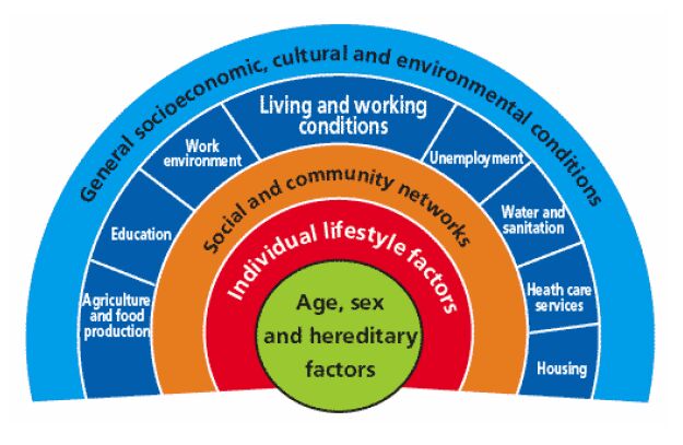
[2] | Dahlgren,G., Whitehead,M. Socioenvironmental model of health. NHS Scotland webpage. 1991. Available from: http://tinyurl.com/a2leomw. |
[3] | EU Member States. Declaration on “Health in All Policies”. Rome: December 2007. Available from: http://tinyurl.com/ok4rx5c. |
[4] | Stone, V (ed.) Health in All Policies. Training Manual (p146). World Health Organisation Geneva. 2015, ISBN 978 92 4 150798 1. Available from: http://tinyurl.com/p7fj2to. |
[5] | Nowacki, J., Martuzzi, M. Capacity Building in Environment and Health (CBEH) Project. Using impact assessment in environment and health: a framework. Copenhagen: WHO Regional Office for Europe, 2013. Available from: http://tinyurl.com/qcl3dyd. |
[6] | Gulis,G., Mekel,O (eds). Assessment of Population Health Risks of Policies. 2014, ISBN 978-1-4614-8597-1 (e-book). Available from: http://tinyurl.com/oylehko. |
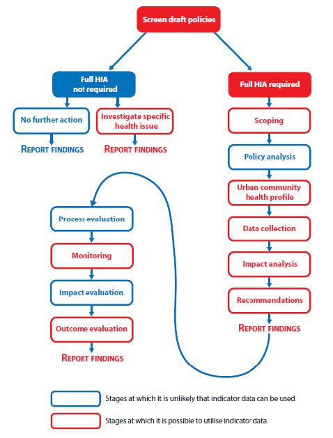
[7] | Dreaves, H et al. Urban Health Impact Assessment Methodology (UrHIA) IMPACT, University of Liverpool. 2015. Available from: http://tinyurl.com/omun9rz . |
[8] | Kemm,J. Developing Health Impact Assessment in Wales. National Assembly for Wales. 1999. Available from: http://tinyurl.com/nctlarv. |
[9] | WHO Regional Office for Europe. Economic cost of the health impact of air pollution in Europe: Clean air, health and wealth. 2015. Available from: http://tinyurl.com/nb7v4dw. |
[10] | Fehr,R et al. Health in Impact Assessments: Opportunities not to be missed. Copenhagen: WHO Regional Office for Europe. 2014. Available from: http://tinyurl.com/ptlguww. |
[11] | Climate and Clean Air Coalition. World Health Assembly passes landmark resolution on air pollution and health. 2015. Available from: http://tinyurl.com/q9zmll4. |
[12] | WHO World Health Assembly. Health and the environment: addressing the health impact of air pollution. Agenda Item 14.6 A68/A/CONF./2 Rev.1 26 May 2015. Available from: http://tinyurl.com/p6w8om4. |
[13] | World Health Organisation. Sixth report of committee A. Draft A68/75. 27 May 2015. Available from: http://tinyurl.com/pnjtqhe. |
[14] | Hawe,P et al. A Framework for building capacity to improve health. New South Wales Health Department. 2001, ISBN 0 7347 3124 8. Available from: http://tinyurl.com/paabjzs. |
[15] | Nowacki, J. Presentation to ESRC Seminar, University of Liverpool, 8th October. 2015. Available from: http://tinyurl.com/q2ksbfj. |
[16] | Birley M. Health Impact Assessment. Principles and Practice. Routledge (e-book). 2011. Available from: http://tinyurl.com/qdwmshf. |
[17] | Commission on the Social Determinants of Health (CSDH). Closing the gap in a generation: health equity through action on the social determinants of health. Final Report of the Commission on Social Determinants of Health. Geneva, World Health Organization. 2008. Available from: http://tinyurl.com/oov72qz. |
[18] | Bell,R., Grobicki, L.,Hamelmann,C. Addressing Social, Economic and Environmental Determinants of Health and the Health Divide in the Context of Sustainable Human Development. UCL Institute of Health Equity for UNDP. 2014. Available from: http://tinyurl.com/negbtyc. |
1. | Xiaojun Yang, Huoxing Li, Ying Sun, Yijie Cai, Hongdi Zhou, Fei Zhong, Research on the Design Method of Cushioning Packaging for Products with Unbalanced Mass, 2023, 13, 2076-3417, 8632, 10.3390/app13158632 |